Simulation setup

Various aspects of the initial conditions for the simulations are described.

Baseline response

The baseline probability/log-odds of treatment success is assumed to vary by silo and site of infection as detailed below.

Baseline probability of treatment success by silo and site of infection

Silo	Joint	Pr(trt success)	log-odds
early	knee	0.65	0.62
early	hip	0.75	1.10
late	knee	0.55	0.20
late	hip	0.6	0.41
chronic	knee	0.6	0.41
chronic	hip	0.65	0.62

Accrual

Accrual is assumed to follow a non-homogeneous Poisson process event times with ramp up over the first 12 months of enrolment and then enrolment of around 1.5 per day.

# events per day
lambda = 1.52
# ramp up over 12 months 
rho = function(t) pmin(t/360, 1)

d_fig <- data.table(
  t = 0:(5 * 365),
  # expected number enrolled
  n = c(0, nhpp.mean(lambda, rho, t1 = 5 * 365, num.points = 5 * 365))
)

ggplot(d_fig, aes(x = t/365, y = n)) +
  geom_line() +
  scale_x_continuous("Year") +
  scale_y_continuous("E[Accrual]", breaks = seq(0, 2500, by = 500))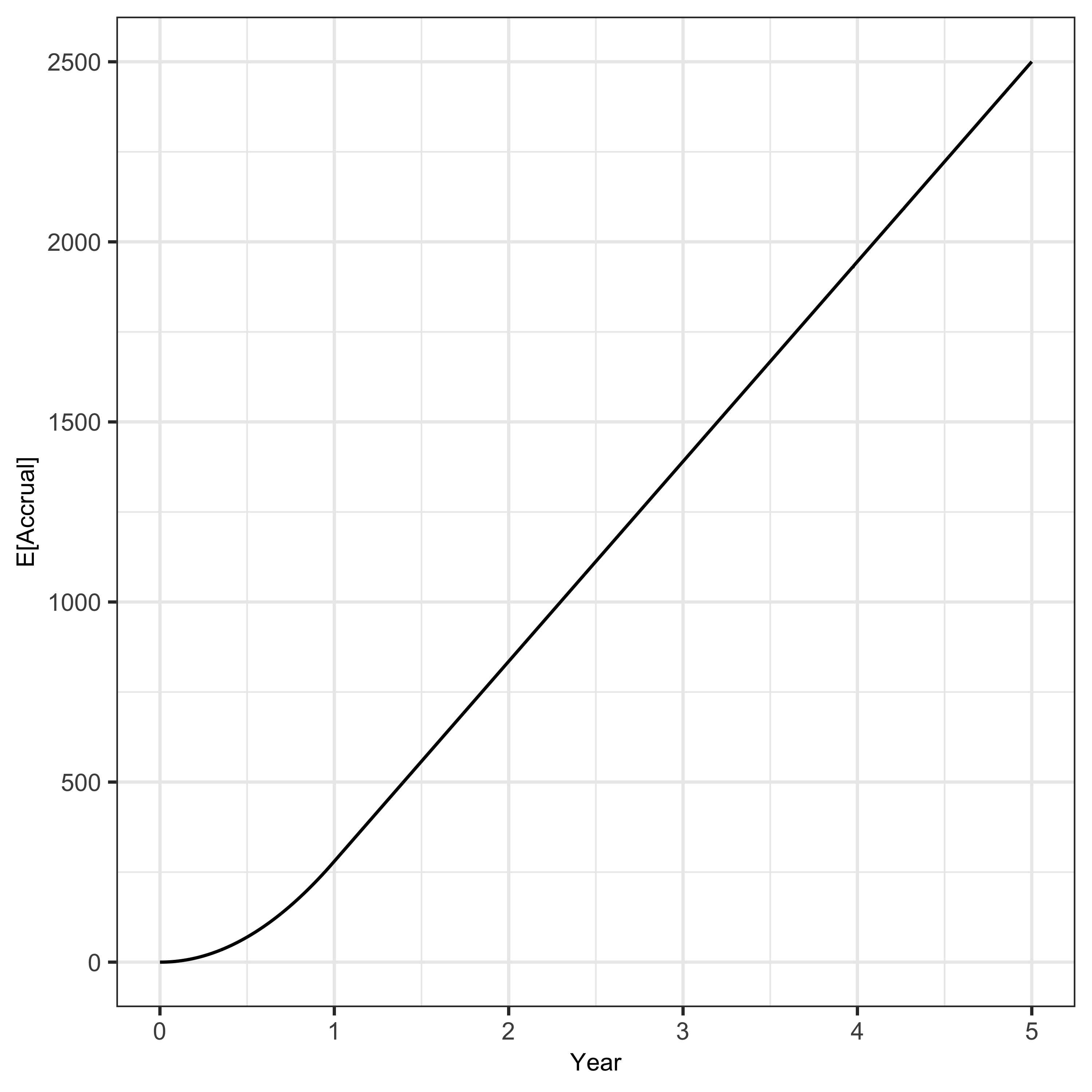

Figure 1: Expected accrual

Domain non-membership effects

We assume a small effects for not being randomised to a domain for all domains.

Missingness

Missingness is not implemented.

Non-differential follow-up

To avoid artifacts associated with non-differential follow-up (e.g. early vs late deaths), participants will be included in the analyses only when they reach the primary endpoints (12 months) irrespective of whether they experienced treatment failure before that time.