Warning: package 'cmdstanr' was built under R version 4.4.3Missingness considerations
Missingness is classed into three types:
- missing completely at random
- missing at random
- missing not at random
which apply to both the response data and covariate data.
The way that you approach the analysis where you have missingness is strongly influenced by the assumptions you can make about the missing data process. Complete case analysis is often chastised but it is sometimes quite a reasonable approach. The following attempts to clarify some of the concepts by way of a simple example.
The following encodes a two-arm parallel group setting where the outcome is treatment failure indicated by \(y = 1\). The data include a treatment group indicator (x), a baseline covariate (a) and an indicator for the presence of adverse event (ae).
We can configure the extent to which the outcome y is influenced by these variables and also how the occurrence of adverse events arises. For example, an adverse event may make the chances of a outcome failure more likely.
Data generation function
get_data <- function(
N = 2000,
par = NULL,
# outcome model
f_y = function(par, x, a, ae){
eta = par$b_out[1] + par$b_out[2]*x + par$b_out[3]*a + par$b_out[4]*ae
eta
},
# model for adverse events
f_ae = function(par, x, a){
eta = par$b_ae[1] + par$b_ae[2]*x + par$b_ae[3]*a
eta
}
){
# strata
d <- data.table()
# intervention - even allocation
d[, x := rbinom(N, 1, par$pr_x)]
# baseline covariate indep to x
d[, a := rbinom(N, 1, par$pr_a)]
# dep on both x and a
d[, eta_ae := f_ae(par, x, a)]
d[, ae := rbinom(.N, 1, plogis(eta_ae))]
# outcome model
d[, eta_y := f_y(par, x, a, ae)]
# y = 1 implies treatment failure
d[, y := rbinom(.N, 1, plogis(eta_y))]
d
}Code
par <- list(
# betas for outcome model (need to align with f_y)
# intervention arm is detrimental (increases the chance of failure)
b_out = c(0.4, 0.3, 0.2, 0.5),
# betas for ae model b0, b_x, b_a (need to align with f_ae)
# intervention arm increases likelihood of ae, as does baseline cov
b_ae = c(-2, 0.5, 0.1),
pr_x = 0.5,
pr_a = 0.7
)
# sanity check/consistency
set.seed(2222222)
d <- get_data(1e6, par)
# align with the outcome model
X <- as.matrix(CJ(x = 0:1, a = 0:1, ae = 0:1))
d_X <- cbind(X, eta = as.numeric(cbind(1, X) %*% par$b_out))
# total effect of exposure (x) on y through all paths
# i.e. possibly through any adverse events as well as the direct path
ate_obs <- coef(glm(y ~ x, data = d, family = binomial))[2]Below is a quick sanity check to see if we can empirically validate the log-odds of the response in each covariate combination.
Code
| Intervention (x) | Covariate | AE Indicator | log-ods response (true) | log-ods response (observed) |
|---|---|---|---|---|
| 0 | 0 | 0 | 0.4 | 0.40 |
| 0 | 0 | 1 | 0.9 | 0.90 |
| 0 | 1 | 0 | 0.6 | 0.60 |
| 0 | 1 | 1 | 1.1 | 1.11 |
| 1 | 0 | 0 | 0.7 | 0.70 |
| 1 | 0 | 1 | 1.2 | 1.18 |
| 1 | 1 | 0 | 0.9 | 0.89 |
| 1 | 1 | 1 | 1.4 | 1.40 |
Missing completely at random
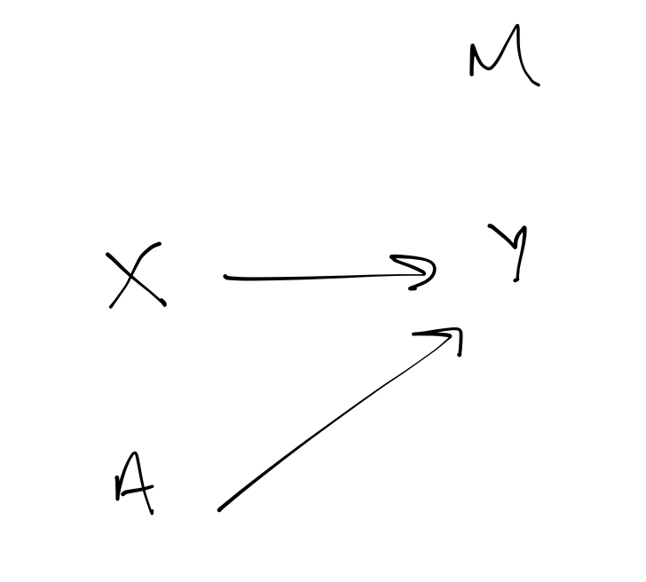
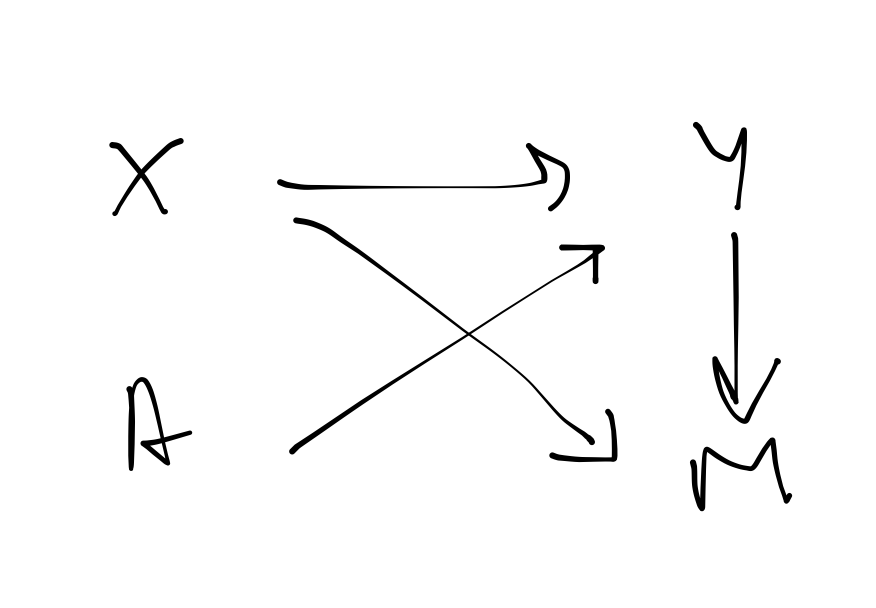
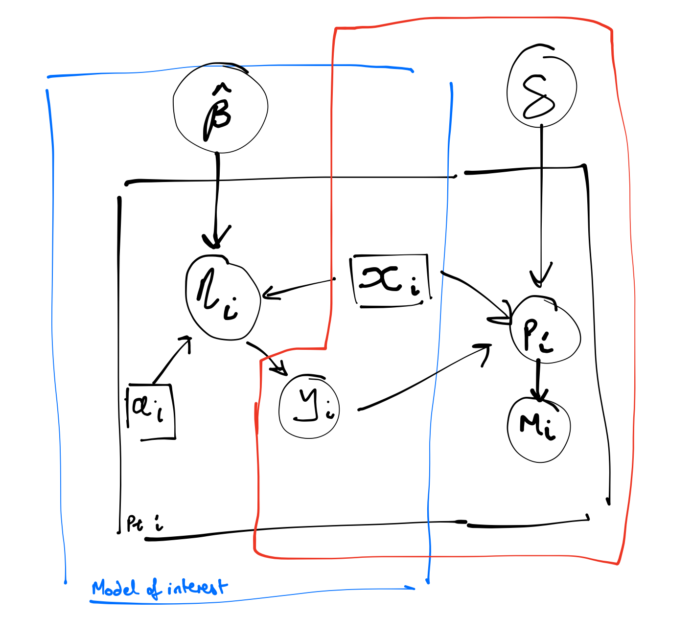
For mcar, the probability of missingness depends on neither the observed or unobserved data. In the Figure 1 (a) DAG, the indicator of missingness (\(m\)) arises as a function of an independent process - it has nothing to do with the observed or unobserved covariates or response and so it sits off by itself as an independent node.
The diagram to the right shows what we might use for the statistical model. The circles show random variables and the squares show observables and the arros show stochastic and logical depdence. The boxes encasing the variables indicate iteration over units.
On the left hand side of the model is the representation of the outcome process. Here y is just a function of \(x\) and \(a\). On the right is the missingness model.
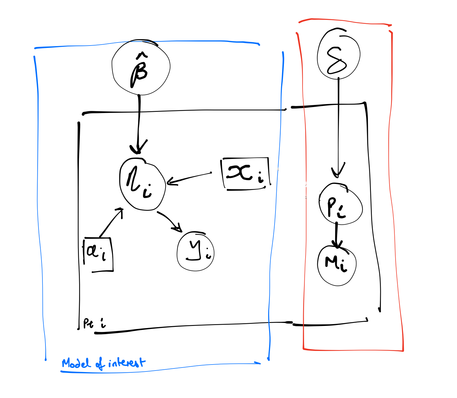
We can incorporate this missing data mechanism into the data simulation. We retain the full data but create an indicator m to tell us which of the rows would be missing.
We would not observe the outcome for those records that were missing (i.e. hose that have \(m=1\)). However, under MCAR, the distribution of the outcome is the same in expectation in the observed and the missing data.
Observed mean response stratified by missingness status
d_fig <- copy(d)
d_fig[, `:=`(x=factor(x, labels = c("ctl", "test")),
a=factor(a, labels = c("<50", ">=50")),
ae=factor(ae, labels = c("no-ae", "ae")),
m = factor(m, labels = c("obs", "mis")))]
d_fig <- d_fig[, .(y = sum(y), n = .N), keyby = .(x, a, m)]
d_fig[, eta_obs := qlogis(y / n)]
ggplot(d_fig,
aes(x= x, y = eta_obs)) +
geom_bar(position="dodge", stat = "identity") +
scale_x_discrete("Exposure") +
scale_y_continuous("log-odds response") +
facet_grid(a ~ m)
Given that the missingness is independent of the outcome, the complete case analysis is unbiased.
Code
d_m <- d[, .(y = sum(y), n = .N), keyby = .(x, a)]
f1_ref <- glm(cbind(y, n-y) ~ x + a, data = d_m, family = binomial)
coef_f1_ref <- summary(f1_ref)$coef
# only select the observed cases
d_m <- d[m == 0, .(y = sum(y), n = .N), keyby = .(x, a)]
f1_cc <- glm(cbind(y, n-y) ~ x + a, data = d_m, family = binomial)
coef_f1_cc <- summary(f1_cc)$coef
d_tbl <- rbind(
data.table(desc = "full data", par = rownames(coef_f1_ref), coef_f1_ref),
data.table(desc = "complete case", par = rownames(coef_f1_cc), coef_f1_cc)
)
d_tbl[, mu_se := sprintf("%.2f (%.3f)", Estimate, `Std. Error`)]
d_tbl[, par := factor(par, levels = c("(Intercept)", "x", "a"))]
knitr::kable(rbind(
dcast(d_tbl, desc ~ par, value.var = "mu_se")
))| desc | (Intercept) | x | a |
|---|---|---|---|
| complete case | 0.41 (0.015) | 0.29 (0.015) | 0.20 (0.016) |
| full data | 0.41 (0.014) | 0.30 (0.013) | 0.19 (0.015) |
We can use multiple imputation (which assumes MAR) for both the MAR and MCAR setting (the latter being a special case of the former). The mice package will default to predicting missing columns on all other variables in the data in line with attempting to maximal uncertainty. We can see that there isn’t really any benefit to imputation if the missing data mechanism is MCAR.
Code
m1 <- cmdstanr::cmdstan_model("stan/missing-ex-01.stan")
d <- get_data(
1e5, par,
f_y = function(par, x, a, ae){
eta = par$b_out[1] + par$b_out[2]*x + par$b_out[3]*a
eta
})
# missingness is indep process
d[, m := rbinom(.N, 1, 0.2)]
d_bin <- d[, .(y = sum(y), n = .N), keyby = .(x, a)]
# full data
ld <- list(
N_obs = nrow(d_bin),
y = d_bin[, y], n = d_bin[, n], P = 3,
X_obs = model.matrix(~ x + a, data = d_bin),
prior_only = 0
)
f1_ref <- m1$sample(ld, iter_warmup = 1000, iter_sampling = 1000,
parallel_chains = 2, chains = 2, refresh = 0, show_exceptions = F,
max_treedepth = 10)Running MCMC with 2 parallel chains...
Chain 1 finished in 0.0 seconds.
Chain 2 finished in 0.0 seconds.
Both chains finished successfully.
Mean chain execution time: 0.0 seconds.
Total execution time: 0.2 seconds.Code
d_post_ref <- data.table(f1_ref$draws(variables = "b", format = "matrix"))
d_post_ref[, desc := "full data"]
# d_post_ref[, lapply(.SD, mean), .SDcols = paste0("b[", 1:3, "]")]
d_bin <- d[m == 0, .(y = sum(y), n = .N), keyby = .(x, a)]
# complete case
ld <- list(
N_obs = nrow(d_bin),
y = d_bin[, y], n = d_bin[, n], P = 3,
X_obs = model.matrix(~ x + a, data = d_bin),
prior_only = 0
)
f1_cc <- m1$sample(ld, iter_warmup = 1000, iter_sampling = 1000,
parallel_chains = 2, chains = 2, refresh = 0, show_exceptions = F,
max_treedepth = 10)Running MCMC with 2 parallel chains...
Chain 1 finished in 0.0 seconds.
Chain 2 finished in 0.0 seconds.
Both chains finished successfully.
Mean chain execution time: 0.0 seconds.
Total execution time: 0.1 seconds.Code
d_post_cc <- data.table(f1_cc$draws(variables = "b", format = "matrix"))
d_post_cc[, desc := "complete case"]
# d_post_cc[, lapply(.SD, mean), .SDcols = paste0("b[", 1:3, "]")]
# number that are missing
# d[, .N, keyby = m]
# imputation sets
d_imp <- copy(d[, .(x, a, y, m)])
d_imp[m == 1, y := NA]
d_imp[, m := NULL]
n_imp <- 50
# dumb mice needs factor if you use logreg
d_imp[, `:=`(x = factor(x), a = factor(a), y = factor(y))]
l_imp <- mice(d_imp, m = n_imp,
method = "logreg",
seed = 23109, printFlag = F)
# print(l_imp)
i <- 1
d_post_imp <- rbindlist(mclapply(1:n_imp, function(i){
# pick up the imputed data set
d_cur <- data.table(complete(l_imp, i))
d_cur[, `:=`(x=as.numeric(as.character(x)),
a=as.numeric(as.character(a)),
y=as.numeric(as.character(y)))]
d_bin <- d_cur[, .(y = sum(y), n = .N), keyby = .(x, a)]
# full (imputed) data
ld <- list(
N_obs = nrow(d_bin),
y = d_bin[, y], n = d_bin[, n], P = 3,
X_obs = model.matrix(~ x + a, data = d_bin),
prior_only = 0
)
snk <- capture.output(
f1_imp <- m1$sample(
ld, iter_warmup = 1000, iter_sampling = 1000,
parallel_chains = 2, chains = 2, refresh = 0, show_exceptions = F,
max_treedepth = 10)
)
d_post <- data.table(f1_imp$draws(variables = "b", format = "matrix"))
d_post
}), idcol = "id_imp")
d_post_imp[, desc := "mi"]
# d_post_imp[, lapply(.SD, mean), .SDcols = paste0("b[", 1:3, "]")]Posterior inference on parameters for full data, complete case and MI
d_fig <- rbind(
d_post_ref, d_post_cc, d_post_imp, fill = T
)
d_fig <- melt(d_fig, id.vars = c("desc", "id_imp"))
d_fig[variable == "b[1]", variable := "(Intercept)"]
d_fig[variable == "b[2]", variable := "x"]
d_fig[variable == "b[3]", variable := "a"]
d_fig[, variable := factor(variable, levels = c("(Intercept)", "x", "a"))]
d_fig[, desc := factor(desc, levels = c("full data", "complete case", "mi"))]
ggplot(data = d_fig, aes(x = value, group = desc, col = desc)) +
geom_density() +
geom_vline(
data = d_fig[, .(mu = mean(value)), keyby = .(desc, variable)],
aes(xintercept = mu, group = desc, col = desc)
) +
geom_vline(
data = d_fig[desc == "full data", .(mu = mean(value)), keyby = .(variable)],
aes(xintercept = mu), col = 2, lwd = 0.4
) +
facet_wrap(desc~variable) +
scale_color_discrete("") +
theme(legend.position = "bottom")
Missing at random
For mar, the probability of missingness depends only on the observed data.
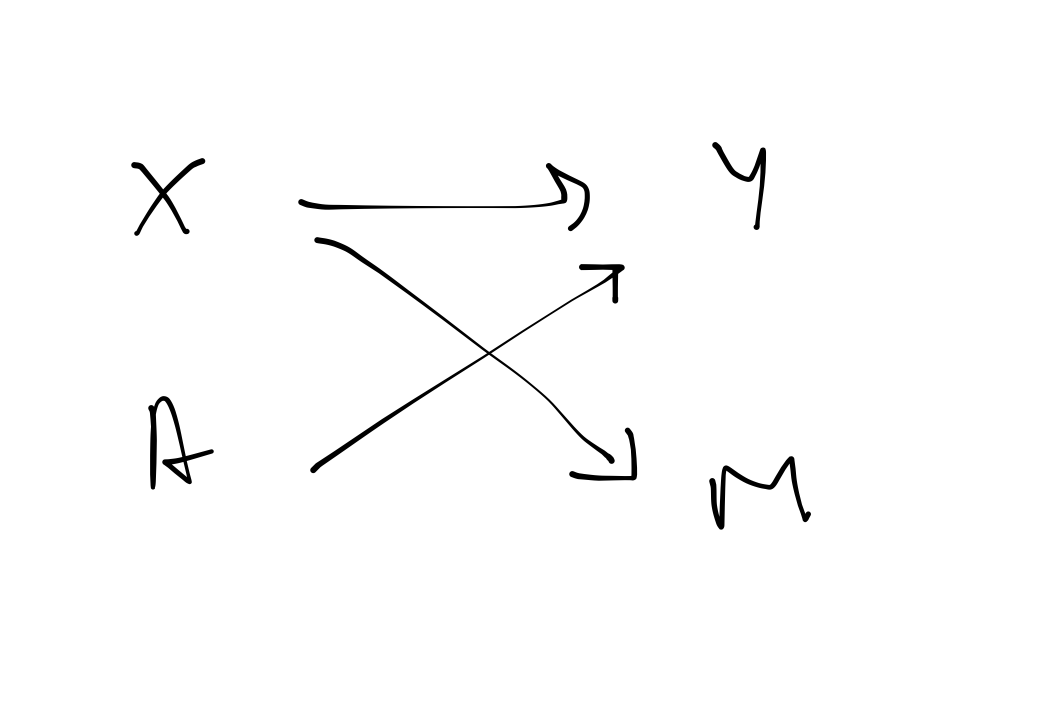
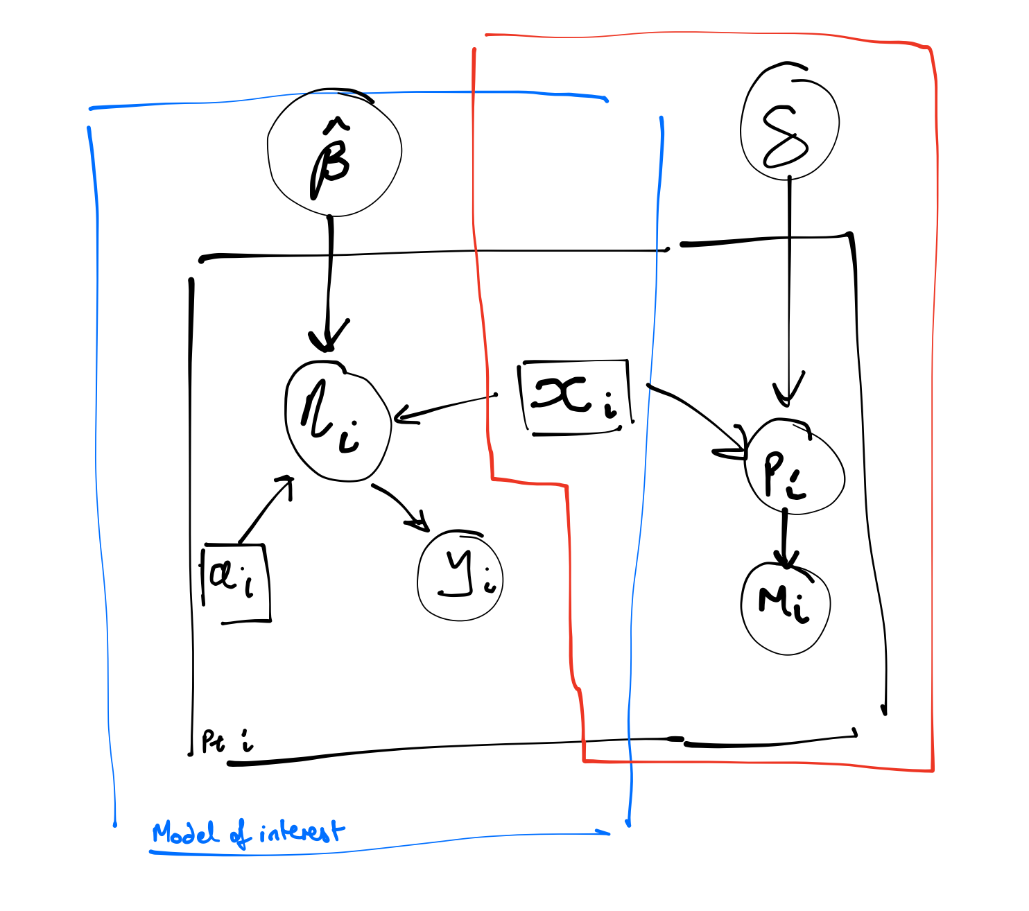
In the Figure 4 (a) DAG, the indicator of missingness arises as a function of the exposure (\(x\)). You could think of this as the possibility of more missingness in the treatment relative to that in the control arm. Again, we would not observe the outcome for those records with \(m=1\). From the DAG you can see that \(y\) and \(m\) are conditionally independent given \(x\). Given that we include \(x\) in the model, the estimates for the treatment effect will be unbiased.
In the simulated data, cross tabulating \(y\) and \(m\) (the observed data and the indicator of missingness) indicates they are dependent.
Pearson's Chi-squared test with Yates' continuity correction
data: d_tbl
X-squared = 115.95, df = 1, p-value < 2.2e-16But when stratified by the exposure and baseline covariates, we cannot conclude any dependence.
Pearson's Chi-squared test with Yates' continuity correction
data: d_tbl
X-squared = 0.16968, df = 1, p-value = 0.6804Conditional on the covariates, the probability of missingness is the same for all levels of the outcome across all strata.
Code
| x | a | trt.success | trt.failure |
|---|---|---|---|
| 0 | 0 | 0.27 | 0.27 |
| 0 | 1 | 0.27 | 0.27 |
| 1 | 0 | 0.73 | 0.73 |
| 1 | 1 | 0.73 | 0.73 |
Which means that the distribution of outcome will be approximately the same in each strata; the missingness is independent of the outcome conditional on the covariates.
Observed mean response stratified by missingness status
d_fig <- copy(d)
d_fig[, `:=`(x=factor(x, labels = c("ctl", "test")),
a=factor(a, labels = c("<50", ">=50")),
ae=factor(ae, labels = c("no-ae", "ae")),
m = factor(m, labels = c("obs", "mis")))]
d_fig <- d_fig[, .(y = sum(y), n = .N), keyby = .(x, a, m)]
d_fig[, eta_obs := qlogis(y / n)]
ggplot(d_fig,
aes(x= x, y = eta_obs)) +
geom_bar(position="dodge", stat = "identity") +
scale_x_discrete("Exposure") +
scale_y_continuous("log-odds response") +
facet_grid(a ~ m)
So, as long as we condition on the predictor of missingness, the complete case estimates are unbiased, albeit inefficient.
Code
d_m <- d[, .(y = sum(y), n = .N), keyby = .(x, a)]
f1_ref <- glm(cbind(y, n-y) ~ x + a, data = d_m, family = binomial)
coef_f1_ref <- summary(f1_ref)$coef
# only select the observed cases
d_m <- d[m == 0, .(y = sum(y), n = .N), keyby = .(x, a)]
f1_cc <- glm(cbind(y, n-y) ~ x + a, data = d_m, family = binomial)
coef_f1_cc <- summary(f1_cc)$coef
d_tbl <- rbind(
data.table(desc = "full data", par = rownames(coef_f1_ref), coef_f1_ref),
data.table(desc = "complete case", par = rownames(coef_f1_cc), coef_f1_cc)
)
d_tbl[, mu_se := sprintf("%.2f (%.3f)", Estimate, `Std. Error`)]
d_tbl[, par := factor(par, levels = c("(Intercept)", "x", "a"))]
knitr::kable(rbind(
dcast(d_tbl, desc ~ par, value.var = "mu_se")
))| desc | (Intercept) | x | a |
|---|---|---|---|
| complete case | 0.41 (0.018) | 0.30 (0.022) | 0.19 (0.020) |
| full data | 0.39 (0.014) | 0.31 (0.013) | 0.21 (0.015) |
Similarly, if the missingness arises because of some baseline covariate, then the estimate for the exposure remains unbiased so long as we adjust for the relevant covariate.
Code
d_m <- d[, .(y = sum(y), n = .N), keyby = .(x, a)]
f1_ref <- glm(cbind(y, n-y) ~ x + a, data = d_m, family = binomial)
coef_f1_ref <- summary(f1_ref)$coef
# only select the observed cases
d_m <- d[m == 0, .(y = sum(y), n = .N), keyby = .(x, a)]
f1_cc <- glm(cbind(y, n-y) ~ x + a, data = d_m, family = binomial)
coef_f1_cc <- summary(f1_cc)$coef
d_tbl <- rbind(
data.table(desc = "full data", par = rownames(coef_f1_ref), coef_f1_ref),
data.table(desc = "complete case", par = rownames(coef_f1_cc), coef_f1_cc)
)
d_tbl[, mu_se := sprintf("%.2f (%.3f)", Estimate, `Std. Error`)]
d_tbl[, par := factor(par, levels = c("(Intercept)", "x", "a"))]
knitr::kable(rbind(
dcast(d_tbl, desc ~ par, value.var = "mu_se")
))| desc | (Intercept) | x | a |
|---|---|---|---|
| complete case | 0.40 (0.017) | 0.29 (0.021) | 0.21 (0.021) |
| full data | 0.39 (0.014) | 0.30 (0.013) | 0.21 (0.014) |
For mcar and mar, the missing data mechanism is referred to as ignorable because we don’t need to specify a model for the missingness in order to make valid inference. We can again use multiple imputation but because we have conditioned the model correctly, there still isn’t any real benefit in the multiple imputation approach.
Code
m1 <- cmdstanr::cmdstan_model("stan/missing-ex-01.stan")
d <- get_data(
1e5, par,
f_y = function(par, x, a, ae){
eta = par$b_out[1] + par$b_out[2]*x + par$b_out[3]*a
eta
})
# missingness is mar
# a function of observed covariates
f_mar <- function(par, x, a){
eta = -1 + 2*x
eta
}
d[, eta_m := f_mar(par, x, a)]
d[, m := rbinom(.N, 1, plogis(eta_m))]
d_bin <- d[, .(y = sum(y), n = .N), keyby = .(x, a)]
# full data
ld <- list(
N_obs = nrow(d_bin),
y = d_bin[, y], n = d_bin[, n], P = 3,
X_obs = model.matrix(~ x + a, data = d_bin),
prior_only = 0
)
f1_ref <- m1$sample(ld, iter_warmup = 1000, iter_sampling = 1000,
parallel_chains = 2, chains = 2, refresh = 0, show_exceptions = F,
max_treedepth = 10)Running MCMC with 2 parallel chains...
Chain 1 finished in 0.0 seconds.
Chain 2 finished in 0.0 seconds.
Both chains finished successfully.
Mean chain execution time: 0.0 seconds.
Total execution time: 0.1 seconds.Code
d_post_ref <- data.table(f1_ref$draws(variables = "b", format = "matrix"))
d_post_ref[, desc := "full data"]
# d_post_ref[, lapply(.SD, mean), .SDcols = paste0("b[", 1:3, "]")]
d_bin <- d[m == 0, .(y = sum(y), n = .N), keyby = .(x, a)]
# complete case
ld <- list(
N_obs = nrow(d_bin),
y = d_bin[, y], n = d_bin[, n], P = 3,
X_obs = model.matrix(~ x + a, data = d_bin),
prior_only = 0
)
f1_cc <- m1$sample(ld, iter_warmup = 1000, iter_sampling = 1000,
parallel_chains = 2, chains = 2, refresh = 0, show_exceptions = F,
max_treedepth = 10)Running MCMC with 2 parallel chains...
Chain 1 finished in 0.0 seconds.
Chain 2 finished in 0.0 seconds.
Both chains finished successfully.
Mean chain execution time: 0.0 seconds.
Total execution time: 0.1 seconds.Code
d_post_cc <- data.table(f1_cc$draws(variables = "b", format = "matrix"))
d_post_cc[, desc := "complete case"]
# d_post_cc[, lapply(.SD, mean), .SDcols = paste0("b[", 1:3, "]")]
# number that are missing
# d[, .N, keyby = m]
# imputation sets
d_imp <- copy(d[, .(x, a, y, m)])
d_imp[m == 1, y := NA]
d_imp[, m := NULL]
# dumb mice needs factor if you use logreg
d_imp[, `:=`(x = factor(x), a = factor(a), y = factor(y))]
n_imp <- 50
l_imp <- mice(d_imp, m = n_imp,
method = "logreg",
seed = 23109, printFlag = F)
# print(l_imp)
i <- 1
d_post_imp <- rbindlist(mclapply(1:n_imp, function(i){
# pick up the imputed data set
d_cur <- data.table(complete(l_imp, i))
d_cur[, `:=`(x=as.numeric(as.character(x)),
a=as.numeric(as.character(a)),
y=as.numeric(as.character(y)))]
d_bin <- d_cur[, .(y = sum(y), n = .N), keyby = .(x, a)]
# full (imputed) data
ld <- list(
N_obs = nrow(d_bin),
y = d_bin[, y], n = d_bin[, n], P = 3,
X_obs = model.matrix(~ x + a, data = d_bin),
prior_only = 0
)
snk <- capture.output(
f1_imp <- m1$sample(
ld, iter_warmup = 1000, iter_sampling = 1000,
parallel_chains = 2, chains = 2, refresh = 0, show_exceptions = F,
max_treedepth = 10)
)
d_post <- data.table(f1_imp$draws(variables = "b", format = "matrix"))
d_post
}), idcol = "id_imp")
d_post_imp[, desc := "mi"]
# d_post_imp[, lapply(.SD, mean), .SDcols = paste0("b[", 1:3, "]")]Posterior inference on parameters for full data, complete case and MI
d_fig <- rbind(
d_post_ref, d_post_cc, d_post_imp, fill = T
)
d_fig <- melt(d_fig, id.vars = c("desc", "id_imp"))
d_fig[variable == "b[1]", variable := "(Intercept)"]
d_fig[variable == "b[2]", variable := "x"]
d_fig[variable == "b[3]", variable := "a"]
d_fig[, variable := factor(variable, levels = c("(Intercept)", "x", "a"))]
d_fig[, desc := factor(desc, levels = c("full data", "complete case", "mi"))]
ggplot(data = d_fig, aes(x = value, group = desc, col = desc)) +
geom_density() +
geom_vline(
data = d_fig[, .(mu = mean(value)), keyby = .(desc, variable)],
aes(xintercept = mu, group = desc, col = desc)
) +
geom_vline(
data = d_fig[desc == "full data", .(mu = mean(value)), keyby = .(variable)],
aes(xintercept = mu), col = 2, lwd = 0.4
) +
facet_wrap(desc~variable) +
scale_color_discrete("") +
theme(legend.position = "bottom")
Missing not at random
If neither mcar or mar hold, then the data are mnar. For mnar, the missing value tells us something about what the value might have been; missingness here is informative, e.g. a salary reporting - people who get paid more tend not to disclose their salary.
Code
d <- get_data(
1e5,
par,
f_y = function(par, x, a, ae){
eta = par$b_out[1] + par$b_out[2]*x + par$b_out[3]*a
eta
})
# missingness is a function of observed covariates and outcome
f_mnar <- function(par, y, x, a){
eta = -1 + 0.5*x + 0.5*y
eta
}
d[, eta_m := f_mnar(par, y, x, a)]
d[, m := rbinom(.N, 1, plogis(eta_m))]The probability of the outcome being missing is now conditional on what would have been observed in the outcome as well as the exposure level with a higher likelihood of missingness in people who would have treatment failure (\(y = 1\) here).
Code
| x | a | trt.success | trt.failure |
|---|---|---|---|
| 0 | 0 | 0.27 | 0.38 |
| 0 | 1 | 0.27 | 0.38 |
| 1 | 0 | 0.38 | 0.50 |
| 1 | 1 | 0.38 | 0.50 |
As a consequence, the distribution of the outcome is no longer same in the observed and the missing data.
Observed mean response stratified by missingness status
d_fig <- copy(d)
d_fig[, `:=`(x=factor(x, labels = c("ctl", "test")),
a=factor(a, labels = c("<50", ">=50")),
ae=factor(ae, labels = c("no-ae", "ae")),
m = factor(m, labels = c("obs", "mis")))]
d_fig <- d_fig[, .(y = sum(y), n = .N), keyby = .(x, a, m)]
d_fig[, eta_obs := qlogis(y / n)]
ggplot(d_fig,
aes(x= x, y = eta_obs)) +
geom_bar(position="dodge", stat = "identity") +
scale_x_discrete("Exposure") +
scale_y_continuous("log-odds response") +
facet_grid(a ~ m)
Now, even after we have conditioned on \(x\) a dependency exists between \(y\) and \(m\). For example, people who have early signs of treatment failure (or success) might choose to leave the study. Under this setting, the treatment effect will generally be biased.
Code
d_m <- d[, .(y = sum(y), n = .N), keyby = .(x, a)]
f1_ref <- glm(cbind(y, n-y) ~ x + a, data = d_m, family = binomial)
coef_f1_ref <- summary(f1_ref)$coef
# only select the observed cases
d_m <- d[m == 0, .(y = sum(y), n = .N), keyby = .(x, a)]
f1_cc <- glm(cbind(y, n-y) ~ x + a, data = d_m, family = binomial)
coef_f1_cc <- summary(f1_cc)$coef
d_tbl <- rbind(
data.table(desc = "full data", par = rownames(coef_f1_ref), coef_f1_ref),
data.table(desc = "complete case", par = rownames(coef_f1_cc), coef_f1_cc)
)
d_tbl[, mu_se := sprintf("%.2f (%.3f)", Estimate, `Std. Error`)]
d_tbl[, par := factor(par, levels = c("(Intercept)", "x", "a"))]
knitr::kable(rbind(
dcast(d_tbl, desc ~ par, value.var = "mu_se")
))| desc | (Intercept) | x | a |
|---|---|---|---|
| complete case | 0.24 (0.017) | 0.24 (0.017) | 0.17 (0.018) |
| full data | 0.40 (0.014) | 0.32 (0.013) | 0.18 (0.014) |
Again, we can try multiple imputation but because MI assumes MAR, things go wrong without some additional assumptions.
Code
m1 <- cmdstanr::cmdstan_model("stan/missing-ex-01.stan")
d <- get_data(
1e5, par,
f_y = function(par, x, a, ae){
eta = par$b_out[1] + par$b_out[2]*x + par$b_out[3]*a
eta
})
# missingness is a function of observed covariates and outcome
f_mnar <- function(par, y, x, a){
eta = -1 + 0.5*x + 0.5*y
eta
}
d[, eta_m := f_mnar(par, y, x, a)]
d[, m := rbinom(.N, 1, plogis(eta_m))]
d_bin <- d[, .(y = sum(y), n = .N), keyby = .(x, a)]
# full data
ld <- list(
N_obs = nrow(d_bin),
y = d_bin[, y], n = d_bin[, n], P = 3,
X_obs = model.matrix(~ x + a, data = d_bin),
prior_only = 0
)
f1_ref <- m1$sample(ld, iter_warmup = 1000, iter_sampling = 1000,
parallel_chains = 2, chains = 2, refresh = 0, show_exceptions = F,
max_treedepth = 10)Running MCMC with 2 parallel chains...
Chain 1 finished in 0.0 seconds.
Chain 2 finished in 0.0 seconds.
Both chains finished successfully.
Mean chain execution time: 0.0 seconds.
Total execution time: 0.1 seconds.Code
d_post_ref <- data.table(f1_ref$draws(variables = "b", format = "matrix"))
d_post_ref[, desc := "full data"]
d_bin <- d[m == 0, .(y = sum(y), n = .N), keyby = .(x, a)]
# complete case
ld <- list(
N_obs = nrow(d_bin),
y = d_bin[, y], n = d_bin[, n], P = 3,
X_obs = model.matrix(~ x + a, data = d_bin),
prior_only = 0
)
f1_cc <- m1$sample(ld, iter_warmup = 1000, iter_sampling = 1000,
parallel_chains = 2, chains = 2, refresh = 0, show_exceptions = F,
max_treedepth = 10)Running MCMC with 2 parallel chains...
Chain 1 finished in 0.0 seconds.
Chain 2 finished in 0.0 seconds.
Both chains finished successfully.
Mean chain execution time: 0.0 seconds.
Total execution time: 0.1 seconds.Code
d_post_cc <- data.table(f1_cc$draws(variables = "b", format = "matrix"))
d_post_cc[, desc := "complete case"]
# number that are missing
# d[, .N, keyby = m]
# imputation sets
d_imp <- copy(d[, .(x, a, y, m)])
d_imp[m == 1, y := NA]
d_imp[, m := NULL]
n_imp <- 50
# dumb mice needs factor if you use logreg
d_imp[, `:=`(x = factor(x), a = factor(a), y = factor(y))]
l_imp <- mice(d_imp, m = n_imp,
method = "logreg",
seed = 23109, printFlag = F)
# print(l_imp)
i <- 1
d_post_imp <- rbindlist(mclapply(1:n_imp, function(i){
# pick up the imputed data set
d_cur <- data.table(complete(l_imp, i))
d_cur[, `:=`(x=as.numeric(as.character(x)),
a=as.numeric(as.character(a)),
y=as.numeric(as.character(y)))]
d_bin <- d_cur[, .(y = sum(y), n = .N), keyby = .(x, a)]
# full (imputed) data
ld <- list(
N_obs = nrow(d_bin),
y = d_bin[, y], n = d_bin[, n], P = 3,
X_obs = model.matrix(~ x + a, data = d_bin),
prior_only = 0
)
snk <- capture.output(
f1_imp <- m1$sample(
ld, iter_warmup = 1000, iter_sampling = 1000,
parallel_chains = 2, chains = 2, refresh = 0, show_exceptions = F,
max_treedepth = 10)
)
d_post <- data.table(f1_imp$draws(variables = "b", format = "matrix"))
d_post
}), idcol = "id_imp")
d_post_imp[, desc := "mi"]Posterior inference on parameters for full data, complete case and MI
d_fig <- rbind(
d_post_ref, d_post_cc, d_post_imp, fill = T
)
d_fig <- melt(d_fig, id.vars = c("desc", "id_imp"))
d_fig[variable == "b[1]", variable := "(Intercept)"]
d_fig[variable == "b[2]", variable := "x"]
d_fig[variable == "b[3]", variable := "a"]
d_fig[, variable := factor(variable, levels = c("(Intercept)", "x", "a"))]
d_fig[, desc := factor(desc, levels = c("full data", "complete case", "mi"))]
ggplot(data = d_fig, aes(x = value, group = desc, col = desc)) +
geom_density() +
geom_vline(
data = d_fig[, .(mu = mean(value)), keyby = .(desc, variable)],
aes(xintercept = mu, group = desc, col = desc)
) +
geom_vline(
data = d_fig[desc == "full data", .(mu = mean(value)), keyby = .(variable)],
aes(xintercept = mu), col = 2, lwd = 0.4
) +
facet_wrap(desc~variable) +
scale_color_discrete("") +
theme(legend.position = "bottom")
A complete case analysis will be unbiased for the treatment effect of interest when the missingness is not depenendent on that term. However, the parameter estimates for the baseline log-odds (intercept) and any term on which the missingness is dependent will be biased.
These results are specific to logistic regression (or more accurately odds ratios, which are a relative measure) and are in contrast to linear regression where the treatment effect will be biased if the missingness is dependent on the outcome regardless of whether adjustment is made. In linear regression the treatment effect from a complete case analysis will be biased if the missingness is due to (1) the outcome alone (2) the outcome and treatment exposure (3) the outcome and baseline factors and is only unbiased under MCAR and when the missingness depends only on the exposure.