Multi-level model perspective

The central idea with modeling discrete heterogeneity in multilevel models is that the variation is assumed to arise within the context of a dependency structure. Under a complete pooling model, the variation is ignored and we assume that the effect is captured within a single parameter such as modeling a treatment effect across groups. For example, consider the model

\[ \begin{aligned} \text{logit}(p_i) &= \alpha + \beta x_i \end{aligned} \]

where \(p\) parameterises a bernoulli observational model conditional on some exposure \(x\) and we are taking a monolithic perspective on the treatment effect. To account for discrete heterogeneity we would replace \(\beta\) with \(\{ \beta_1, \beta_2, \dots \beta_K \}\). However, to complete the model we neeed to place a prior on \(\beta_k\). Under the assumption of no latent interactions (as in no pooling) we would adopt \(\pi(\beta_1, \dots, \beta_K) = \pi_1(\beta_1)\dots\pi_K(\beta_K)\). Under a partial pooling perspective, we would assume some structure to the prior.

REMAP-CAP uses a multilevel perspective for modeling treatment effects within a domain, across strata, that I have translated to the ROADMAP context although I have made some simplifications for the purposes of illustration.

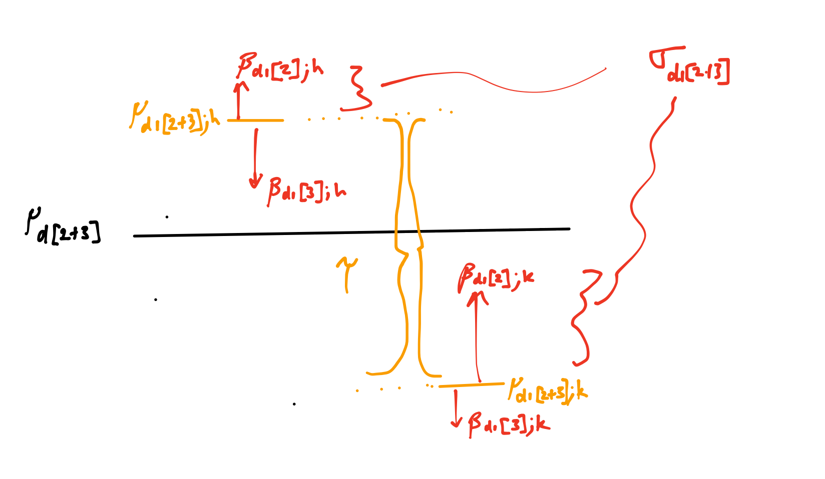
Assume the following structure for the linear predictor

\[ \begin{aligned} \text{logit}(p) &= \beta_0 + \beta_{d1[x], j} \end{aligned} \]

where the second term represents a joint specific effect of exposure \(x\) within the first domain (I am ignoring silo for the moment and treating everything as generic).

The parameters and priors are structured as follows

Parameters and priors

Parameter	Domain	Joint	Prior	Note
\(\beta_{[d1[1];j]}\)	Surgery	knee,hip	0	Randomised DAIR (ref for rand comparisons)
\(\beta_{[d1[2];j]}\)	Surgery	knee,hip	\(N(\mu_{[d1[2+3];j]}, \sigma_{[d1[2+3]]})\)	Randomised REV (one-stage selected)
\(\beta_{[d1[3];j]}\)	Surgery	knee,hip	\(N(\mu_{[d1[2+3];j]}, \sigma_{[d1[2+3]]})\)	Randomised REV (two-stage selected)
\(\mu_{[d1[2+3];j]}\)	Surgery	knee,hip	\(N(\mu_{[d1[2+3]]}, \tau_{[d1[2+3]]})\)	Mean revision effect by joint
\(\mu_{[d1[2+3]]}\)	Surgery	knee,hip	\(N(0, 1)\)	Overall mean of revision effect
\(\tau_{[d1[2+3]]}\)	Surgery		\(\text{Student}(3,0,2)\)	SD across joint variation
\(\sigma_{[d1[2+3]]}\)	Surgery		\(\text{Student}(3,0,2)\)	SD within joint variation

The idea is to produce a structure whereby estimation of the variance components produces dynamic shrinkage of the treatment effect estimates.

Revision effects

Specifically, when the variance components are estimated to be large then more variation in the strata specific treatment effects is permitted. However, to estimate the variance components well, you will need multiple groups (more than two).

Example - large number of groups and exposure levels

For the sake of an example, assume you have a setting with 8 treatment arms to which patients are randomised and within each treatment arm are a mix of participants with respect to some characteristic that could influence the response. I am only using this many treatment arms because it allows us to see a clear difference between the different analysis approaches. We are interested in the overall treatment effect and heterogeneity due to some membership to a group.

Within this setting there are multiple levels of variation. There is the between treatment arm variation that characterises how different the treatment arms are. There is also the within treatment arm variation due to the subgroup.

We could adopt a range of assumptions to model the responses for each combination of treatment and subgroup.

1. Model the responses for each treatment arm by subgroup combination independently; no information is shared between any of the combinations. This approach will recover the observed point estimates and could be achieved using a logistic regression to estimate each combination’s mean response.
2. Model the treatment groups independently, but estimate the variation within each treatment arm due to subgroup membership by sharing a common variance parameter across all the treatment arms. This will reflect the observed mean response in each treatment arm but shrink the subgroup variation towards these means. It will only do this if there is sufficient data to inform the relevant variance estimate.
3. Model both the between treatment arm variation and the within treatment arm variation by partitioning the total variation. This will tend to shrink the treatment arm means towards an overall mean and the subgroup estimates towards each treatment arm mean. The within group variation could be modelled for each treatment arm independently or be shared across all treatments.

Plus variations on these themes. All of the variance partition approaches require that there are sufficient groups to informed the variance parameters.

Here I assume the following represents the true model

\[ \begin{aligned} y_{ijk} &\sim \text{Bernoulli}(\text{logit}^{-1}(\nu_{jk})) \\ \nu_{jk} &\sim \text{Normal}(\delta_j, \tau) \\ \delta_j &\sim \text{Normal}(\mu, \sigma) \end{aligned} \]

and adopt hyper priors and hyper parameters

\[ \begin{aligned} \mu &\sim \text{Normal}(0, 1) \\ \tau &\sim \text{Student-t}(\text{df} = 3,0, \text{scale} = 2) \\ \sigma &\sim \text{Student-t}(3,0,2) \\ \end{aligned} \]

Parameter specification/generation

Assume that the true treatment group means are normally distributed around some non-zero mean with standard deviation \(s\) and that the subgroup means are normally distributed around each treatment group mean with a common standard deviation \(s_j\).

get_par <- function(
    n_grp = 4, n_trt = 9,
    mu = 1,
    s = 0.1, s_j = 0.3
    ){
  
  l <- list()
  l$n_grp <- n_grp
  l$n_trt <- n_trt

  # overall mean effect across all intervention types
  l$mu <- mu
  # between intervention type variation
  l$s <- s
  # intervention type specific mean
  l$mu_j <- l$mu + rnorm(n_trt, 0, l$s)
  # within intervention variation attributable to group membership
  l$s_j <- s_j

  # trt x group effects
  l$mu_j_k <- do.call(rbind, lapply(seq_along(l$mu_j), function(i){
    rnorm(n_grp, l$mu_j[i], l$s_j)
  }))
  colnames(l$mu_j_k) <- paste0("strata", 1:ncol(l$mu_j_k))
  rownames(l$mu_j_k) <- paste0(1:nrow(l$mu_j_k))
  
  l$d_par <- CJ(
    j = factor(1:l$n_trt, levels = 1:l$n_trt),
    k = factor(1:l$n_grp, levels = 1:l$n_grp)
  )
  l$d_par[, mu := l$mu]
  l$d_par[, mu_j := l$mu_j[j]]
  l$d_par[, mu_j_k := l$mu_j_k[cbind(j,k)]]
  
  l
}

Any single data set will not allow us to recover the parameters exactly, but the differences between the estimates from the various modelling assumptions is informative as to the general patterns that arise.

get_data <- function(
    N = 2000, 
    par = NULL,
    ff = function(par, j, k){
      
      m1 <- cbind(j, k)
      eta = par$mu_j_k[m1] 
      eta
      
    }){
  
  # strata
  d <- data.table()
  
  # intervention - even allocation
  d[, j := sample(1:par$n_trt, size = N, replace = T)]
  # table(d$j)
  # uneven distribution of groups in the pop
  z <- rnorm(par$n_grp, 0, 0.5)
  d[, k := sample(1:par$n_grp, size = N, replace = T, prob = exp(z)/sum(exp(z)))]
  # d[, k := sample(1:par$n_grp, size = N, replace = T)]
  # table(d$j, d$k)
  
  d[, eta := ff(par, j, k)]
  
  d[, y := rbinom(.N, 1, plogis(eta))]
  
  d  
}

Generate data assuming the parameters below with the underlying truth shown in Figure 1. The dashed line shows the overall mean response, the crosses show the treatment arm means and the points show the subgroup heterogeneity around the treatment arm means. Within this first setup, all the treatment arms have the same response and none of the subgroups show any treatment effect either.

set.seed(1)
par <- get_par(n_grp = 5, n_trt = 8, mu = 1, s = 0.0, s_j = 0)
d <- get_data(N = 3000, par)


d_fig_2 <- unique(par$d_par[, .(mu_j, j)])
d_fig_2[1, label := "Treatment mean"]
       
d_fig_3 <- copy(par$d_par)
d_fig_3[6, label := "Subgroup mean"]


p_fig <- ggplot(d_fig_3, aes(x = j, y = mu_j_k, col = k)) +
  geom_jitter(width = 0.2, height = 0.01) +
  geom_hline(yintercept = par$mu, lwd = 0.25, lty = 2) +
  geom_text_repel(
    aes(label = label),
                  nudge_x = 0.5,
                  nudge_y = -0.2,
                  segment.curvature = -0.1,
                  segment.ncp = 3,
                  segment.angle = 20,
                  box.padding = 2, max.overlaps = Inf, col = 1) +
  geom_text_repel(
    data = data.table(
      x = 2.5, y = par$mu, label = "Overall mean"
    ),
    aes(x = x, y = y, label = label),
                  inherit.aes = F,
                  nudge_x = 0.4,
                  nudge_y = 0.1,
                  segment.curvature = -0.1,
                  segment.ncp = 3,
                  segment.angle = 20,
                  box.padding = 2, max.overlaps = Inf, col = 1) +
  geom_text_repel(data = d_fig_2,
                  aes(x = j, y = mu_j, label = label), 
                  inherit.aes = F,
                  nudge_x = 0.4,
                  nudge_y = -0.05,
                  segment.curvature = -0.1,
                  segment.ncp = 3,
                  segment.angle = 20,
                  box.padding = 2, max.overlaps = Inf, col = 1) +
  geom_point(data = d_fig_2,
             aes(x = j, y = mu_j),
             inherit.aes = F, pch = 3, size = 3) +
  scale_x_discrete("Treatment type") +
  scale_y_continuous("Odds of success (log-odds)", 
                     breaks = seq(
                       0.5, 
                       1.5, 
                       by = 0.1), limits = c(0.5, 1.5)) +
  scale_color_discrete("Subgroup membership")

suppressWarnings(print(p_fig))

Figure 1: True treatment arm by subgroup mean response

Parameter estimation

Below are models that provide the observed, ML, unpooled and partially pooled estimates.

# mle - reference point
d_lm <- copy(d)
d_lm[, `:=`(j = factor(j), k = factor(k))]
f0 <- glm(y ~ j*k, data = d_lm, family = binomial)
X <- model.matrix(f0)
# CI
n_sim <- 1000
d_lm_j <- matrix(NA, nrow = par$n_trt, ncol = n_sim)
d_lm_j_k <- matrix(NA, nrow = par$n_trt * par$n_grp, ncol = n_sim)
for(i in 1:n_sim){
  ix <- sort(sample(1:nrow(d_lm), replace = T))
  f_boot <- glm(y ~ j*k, data = d_lm[ix], family = binomial)
  d_tmp_p <- cbind(
    d_lm[ix],
    mu = predict(f_boot)
  )
  d_lm_j[, i] <- d_tmp_p[, .(mean = mean(mu)), keyby = j][, mean]
  d_lm_j_k[, i] <- d_tmp_p[, .(mean = mean(mu)), keyby = .(k, j)][, mean]
}
# bootstrapped intervals for means on j and within group means
d_lm_j <- data.table(d_lm_j)
d_lm_j[, j := 1:.N]
d_lm_j <- melt(d_lm_j, id.vars = "j")
d_lm_j[, j := factor(j)]
# d_lm_j[, .(q5 = quantile(value, prob =0.05), 
#            q95 = quantile(value, prob = 0.95)), keyby = j]

d_lm_j_k <- data.table(d_lm_j_k)
d_lm_j_k <- cbind(CJ(k = 1:par$n_grp, j = 1:par$n_trt), d_lm_j_k)
d_lm_j_k <- melt(d_lm_j_k, id.vars = c("j", "k"))
d_lm_j_k[, `:=`(j = factor(j), k = factor(k))]
# d_lm_j_k[, .(q5 = quantile(value, prob =0.05), 
#            q95 = quantile(value, prob = 0.95)), keyby = .(k,j)]
d_lm[, eta_hat := predict(f0)]

# bayes
m1 <- cmdstanr::cmdstan_model("stan/mlm-ex-01.stan")
m2 <- cmdstanr::cmdstan_model("stan/mlm-ex-02.stan")
m3 <- cmdstanr::cmdstan_model("stan/mlm-ex-03.stan")

ld <- list(
  N = nrow(d), 
  y = d$y, 
  J = length(unique(d$j)), K = length(unique(d$k)),
  j = d$j, # intervention
  k = d$k, # subgroup
  P = ncol(X),
  X = X,
  s = 3,
  s_j = 3, # for the indep means offsets
  prior_only = 0
)

f1 <- m1$sample(
    ld, iter_warmup = 1000, iter_sampling = 1000,
    parallel_chains = 2, chains = 2, refresh = 0, show_exceptions = F,
    max_treedepth = 10)

Running MCMC with 2 parallel chains...

Chain 2 finished in 7.7 seconds.
Chain 1 finished in 9.3 seconds.

Both chains finished successfully.
Mean chain execution time: 8.5 seconds.
Total execution time: 9.4 seconds.

f2 <- m2$sample(
    ld, iter_warmup = 1000, iter_sampling = 1000,
    parallel_chains = 2, chains = 2, refresh = 0, show_exceptions = F,
    max_treedepth = 10)

Running MCMC with 2 parallel chains...

Chain 1 finished in 2.1 seconds.
Chain 2 finished in 2.1 seconds.

Both chains finished successfully.
Mean chain execution time: 2.1 seconds.
Total execution time: 2.2 seconds.

f3 <- m3$sample(
    ld, iter_warmup = 1000, iter_sampling = 1000,
    parallel_chains = 2, chains = 2, refresh = 0, show_exceptions = F,
    max_treedepth = 10)

Running MCMC with 2 parallel chains...

Chain 1 finished in 2.4 seconds.
Chain 2 finished in 2.4 seconds.

Both chains finished successfully.
Mean chain execution time: 2.4 seconds.
Total execution time: 2.6 seconds.

Figure 2 shows the estimated treatment arm means. The mlm correctly identifies the absence of between treatment variation and as a result, the means are pulled towards the grand mean.

d_1 <- data.table(t(f1$draws(variables = "eta", format = "matrix")))
d_1 <- cbind(d, d_1)
d_1 <- melt(d_1, id.vars = c("j", "k", "eta", "y"), variable.name = "i_draw")

d_2 <- data.table(t(f2$draws(variables = "eta", format = "matrix")))
d_2 <- cbind(d, d_2)
d_2 <- melt(d_2, id.vars = c("j", "k", "eta", "y"), variable.name = "i_draw")

d_3 <- data.table(t(f3$draws(variables = "eta", format = "matrix")))
d_3 <- cbind(d, d_3)
d_3 <- melt(d_3, id.vars = c("j", "k", "eta", "y"), variable.name = "i_draw")

d_mu_j <- rbind(
  d_1[, .(mu = mean(value)), keyby = .(j, i_draw)][
  , .(desc = "no pooling", 
      mean = mean(mu), 
      q5 = quantile(mu, prob = 0.05), 
      q95 = quantile(mu, prob = 0.95)), keyby = j],
  d_2[, .(mu = mean(value)), keyby = .(j, i_draw)][
  , .(desc = "partial pool (trt)", 
      mean = mean(mu), 
      q5 = quantile(mu, prob = 0.05), 
      q95 = quantile(mu, prob = 0.95)), keyby = j],
  d_3[, .(mu = mean(value)), keyby = .(j, i_draw)][
  , .(desc = "partial pool (trt+subgrp)", 
      mean = mean(mu), 
      q5 = quantile(mu, prob = 0.05), 
      q95 = quantile(mu, prob = 0.95)), keyby = j]
)
  

# MLE
d_mle <- cbind(
  desc = "mle", 
  d_lm[, .(mean = mean(eta_hat)), keyby = .(j)])
d_mle <- merge(
  d_mle, 
  d_lm_j[, .(q5 = quantile(value, prob =0.05),
           q95 = quantile(value, prob = 0.95)), keyby = j], 
  by = "j"
)

d_mu_j <- rbind(d_mu_j, d_mle, fill = T)

# Observed
# Due to the imbalance between the subgroups, need to weight the
# contributions to align (approx) with mle.
# Easy here because only one other variable that we need to average
# over.
d_obs <- merge(
  d[, .(N_j = .N), keyby = .(j)],
  d[, .(mu = qlogis(mean(y)), .N), keyby = .(j, k)],
  by = "j"
)
d_mu_j <- rbind(
  d_mu_j,
  d_obs[, .(
    desc = "observed", 
    mean = sum(mu * N / N_j)), keyby = j]
  , fill = T
  )


d_mu_j[, desc := factor(desc, levels = c(
  "observed", "mle", "no pooling", 
  "partial pool (trt)", "partial pool (trt+subgrp)"
))]
  


d_mu <- d[, .(mu = qlogis(mean(y)), 
         w = .N/nrow(d)), keyby = .(j, k)][
           , .(desc = "observed", mean = sum(mu * w))]


p_fig <- ggplot(d_mu_j, aes(x = j, y = mean, group = desc, col = desc)) +
  geom_point(position = position_dodge(width = 0.6)) +
  geom_linerange(aes(ymin=q5, ymax=q95), position = position_dodge2(width = 0.6)) +
  geom_hline(data = d_mu,
             aes(yintercept = mean, lty = desc),
             lwd = 0.3, col = 1) +
  scale_x_discrete("Treatment arm") +
  scale_y_continuous("log-odds treatment success", breaks = seq(-3, 3, by = 0.2))  +
  scale_color_discrete("") +
  scale_linetype_discrete("") +
  geom_text(data = d[, .N, keyby = .(j)],
            aes(x = j, y = min(d_mu_j$q5, na.rm = T) - 0.1, 
                label = N), inherit.aes = F) +
  theme(legend.position="bottom", legend.box="vertical", legend.margin=margin())

suppressWarnings(print(p_fig))  

Figure 2: Parameter estimates vs true values

Figure 3 shows the estimated treatment by subgroup means. Similar to above, the mlm has determined that the within group variance is negligible and has pulled the subgroup estimates towards the treatment means. In contrast, the ML and independent models follow the data leading to suggest some material subgroup effects.

# Posterior
# d_mu_j_k <- rbind(
#   data.table(f2$summary(variables = c(
#     "mu_j_k"
#     )))[, .(desc = "partial pool (trt)", variable, mean, q5, q95)],
#   data.table(f3$summary(variables = c(
#     "mu_j_k"
#     )))[, .(desc = "partial pool (trt+subgrp)", variable, mean, q5, q95)]
# )
# d_mu_j_k[, j := substr(variable, 8, 8)]
# d_mu_j_k[, k := substr(variable, 10, 10)]

# Manually calculate intervals for independent model
d_mu_j_k <- rbind(
  # d_mu_j_k,
  d_1[, .(mu = mean(value)), keyby = .(k, j, i_draw)][
  , .(desc = "no pooling", 
      mean = mean(mu), 
      q5 = quantile(mu, prob = 0.05), 
      q95 = quantile(mu, prob = 0.95)), keyby = .(k, j)],
  d_2[, .(mu = mean(value)), keyby = .(k, j, i_draw)][
  , .(desc = "partial pool (trt)", 
      mean = mean(mu), 
      q5 = quantile(mu, prob = 0.05), 
      q95 = quantile(mu, prob = 0.95)), keyby = .(k, j)],
  d_3[, .(mu = mean(value)), keyby = .(k, j, i_draw)][
  , .(desc = "partial pool (trt+subgrp)", 
      mean = mean(mu), 
      q5 = quantile(mu, prob = 0.05), 
      q95 = quantile(mu, prob = 0.95)), keyby = .(k, j)]
  )

# MLE
d_mle <- cbind(
  desc = "mle", 
  d_lm[, .(mean = mean(eta_hat)), keyby = .(k, j)])
d_mle <- merge(
  d_mle, 
  d_lm_j_k[, .(q5 = quantile(value, prob =0.05),
               q95 = quantile(value, prob = 0.95)), keyby = .(k,j)], 
  by = c("j","k")
)

d_mu_j_k <- rbind(d_mu_j_k, d_mle, fill = T)

# Observed
d_mu_j_k <- rbind(
  d_mu_j_k, 
  d[, .(desc = "observed", mean = qlogis(mean(y))), keyby = .(k, j)],
  fill = T)


d_mu_j_k[, desc := factor(desc, levels = c(
  "observed", "mle", "no pooling", "partial pool (trt)", "partial pool (trt+subgrp)"
))]

# 
d_mu_obs <- d[, .(mu = qlogis(mean(y)))]
d_mu_mod <- data.table(f3$summary(variables = c(
    "mu"
    )))[, .(model = "no pooling", variable, mean, q5, q95)]

p_fig <- ggplot(d_mu_j_k, aes(x = k, y = mean, group = desc, col = desc)) +
  geom_point(position = position_dodge(width = 0.6)) +
  geom_linerange(aes(ymin=q5, ymax=q95), position = position_dodge2(width = 0.6)) +
  scale_x_discrete("Subgroup") +
  scale_y_continuous("log-odds treatment success", breaks = seq(-3, 3, by = 0.2)) +
  geom_hline(data = d_mu_j[desc == "observed"],
             aes(yintercept = mean, group = desc),
             lwd = 0.3, col = 1) +
  geom_text(data = d[, .N, keyby = .(j, k)],
            aes(x = k, y = min(d_mu_j_k$q5, na.rm = T) - 0.1, label = N), 
            inherit.aes = F) +
  facet_wrap(~paste0("Treatment ", j)) 

suppressWarnings(print(p_fig))

Figure 3: Parameter estimates vs true values

The mlm partitions the variance into a between treatment variance part that characterises the variation in the treatment arms and a within treatment variance that characterises the variation due to the subgroups.

In Figure 4 shows the prior (red) and the posterior (black) for the variance components (actually the standard deviations). Given the differentiation between the prior and posterior, it is clear that something has been learnt about the variation in the data and the posterior is well identified, although not fully concentrated on the true value of zero. Moreover, both the between group variation (variation due to treatment) and within group variation (variation due to subgroups) are small which leads to the dynamic shrinkage as shown in the subgroup level means.

d_fig <- rbind(
  cbind(desc = "partial pool (trt)",
        data.table(f2$draws(variables = c("s_j"), format = "matrix"))),
  cbind(desc = "partial pool (trt+subgrp)",
        data.table(f3$draws(variables = c("s", "s_j"), format = "matrix"))  
  ), fill = T
)
d_fig <- melt(d_fig, id.vars = "desc")
d_fig[variable == "s", label := "variation b/w"]
d_fig[variable == "s_j", label := "variation w/in"]

d_pri <- CJ(
  variable = c("s", "s_j"),
  desc = c("partial pool (trt)", "partial pool (trt+subgrp)"),
  x = seq(min(d_fig$value, na.rm = T), 
          max(d_fig$value, na.rm = T), len = 500)
)
d_pri[, y := fGarch::dstd(x, nu = 3, mean = 0, sd = 2)]
d_pri[variable == "s", label := "variation b/w"]
d_pri[variable == "s_j", label := "variation w/in"]
d_pri[desc == "partial pool (trt)" & variable == "s", y := NA]
# 
# d_smry <- d_fig[, .(mu = mean(value)), keyby = .(label)]

p_fig <- ggplot(d_fig, aes(x = value, group = variable)) + 
  geom_density() +
  geom_line(
    data = d_pri, 
    aes(x = x, y = y), col = 2, lwd = 0.2
  ) +
  scale_x_continuous("Standard deviation") +
  scale_y_continuous("Density") +
  facet_wrap(desc+label~., ncol = 2)

suppressWarnings(print(p_fig))

Figure 4: Between and within SD

Example - small number of groups and exposure levels

Now repeat the same exercise with a small number of groups and exposure levels, again we simulate the data assuming no effects are present.

set.seed(1)
par <- get_par(n_grp = 2, n_trt = 2, mu = 1, s = 0.0, s_j = 0.0)
d <- get_data(N = 3000, par)

# mle - reference point
d_lm <- copy(d)
d_lm[, `:=`(j = factor(j), k = factor(k))]
f0 <- glm(y ~ j*k, data = d_lm, family = binomial)
X <- model.matrix(f0)
# CI
n_sim <- 1000
d_lm_j <- matrix(NA, nrow = par$n_trt, ncol = n_sim)
d_lm_j_k <- matrix(NA, nrow = par$n_trt * par$n_grp, ncol = n_sim)
for(i in 1:n_sim){
  ix <- sort(sample(1:nrow(d_lm), replace = T))
  f_boot <- glm(y ~ j*k, data = d_lm[ix], family = binomial)
  d_tmp_p <- cbind(
    d_lm[ix],
    mu = predict(f_boot)
  )
  d_lm_j[, i] <- d_tmp_p[, .(mean = mean(mu)), keyby = j][, mean]
  d_lm_j_k[, i] <- d_tmp_p[, .(mean = mean(mu)), keyby = .(k, j)][, mean]
}
# bootstrapped intervals for means on j and within group means
d_lm_j <- data.table(d_lm_j)
d_lm_j[, j := 1:.N]
d_lm_j <- melt(d_lm_j, id.vars = "j")
d_lm_j[, j := factor(j)]
# d_lm_j[, .(q5 = quantile(value, prob =0.05), 
#            q95 = quantile(value, prob = 0.95)), keyby = j]

d_lm_j_k <- data.table(d_lm_j_k)
d_lm_j_k <- cbind(CJ(k = 1:par$n_grp, j = 1:par$n_trt), d_lm_j_k)
d_lm_j_k <- melt(d_lm_j_k, id.vars = c("j", "k"))
d_lm_j_k[, `:=`(j = factor(j), k = factor(k))]
# d_lm_j_k[, .(q5 = quantile(value, prob =0.05), 
#            q95 = quantile(value, prob = 0.95)), keyby = .(k,j)]

d_lm[, eta_hat := predict(f0)]

# bayes
m1 <- cmdstanr::cmdstan_model("stan/mlm-ex-01.stan")
m2 <- cmdstanr::cmdstan_model("stan/mlm-ex-02.stan")
m3 <- cmdstanr::cmdstan_model("stan/mlm-ex-03.stan")

ld <- list(
  N = nrow(d), 
  y = d$y, 
  J = length(unique(d$j)), K = length(unique(d$k)),
  j = d$j, # intervention
  k = d$k, # subgroup
  P = ncol(X),
  X = X,
  s = 3,
  s_j = 3, # for the indep means offsets
  prior_only = 0
)

f1 <- m1$sample(
    ld, iter_warmup = 1000, iter_sampling = 1000,
    parallel_chains = 2, chains = 2, refresh = 0, show_exceptions = F,
    max_treedepth = 10)

Running MCMC with 2 parallel chains...

Chain 1 finished in 1.4 seconds.
Chain 2 finished in 1.5 seconds.

Both chains finished successfully.
Mean chain execution time: 1.4 seconds.
Total execution time: 1.6 seconds.

f2 <- m2$sample(
    ld, iter_warmup = 1000, iter_sampling = 1000,
    parallel_chains = 2, chains = 2, refresh = 0, show_exceptions = F,
    max_treedepth = 10)

Running MCMC with 2 parallel chains...

Chain 1 finished in 2.3 seconds.
Chain 2 finished in 2.7 seconds.

Both chains finished successfully.
Mean chain execution time: 2.5 seconds.
Total execution time: 2.8 seconds.

Warning: 22 of 2000 (1.0%) transitions ended with a divergence.
See https://mc-stan.org/misc/warnings for details.

f3 <- m3$sample(
    ld, iter_warmup = 1000, iter_sampling = 1000,
    parallel_chains = 2, chains = 2, refresh = 0, show_exceptions = F,
    max_treedepth = 10)

Running MCMC with 2 parallel chains...

Chain 1 finished in 5.0 seconds.
Chain 2 finished in 6.0 seconds.

Both chains finished successfully.
Mean chain execution time: 5.5 seconds.
Total execution time: 6.1 seconds.

Warning: 57 of 2000 (3.0%) transitions ended with a divergence.
See https://mc-stan.org/misc/warnings for details.

d_1 <- data.table(t(f1$draws(variables = "eta", format = "matrix")))
d_1 <- cbind(d, d_1)
d_1 <- melt(d_1, id.vars = c("j", "k", "eta", "y"), variable.name = "i_draw")

d_2 <- data.table(t(f2$draws(variables = "eta", format = "matrix")))
d_2 <- cbind(d, d_2)
d_2 <- melt(d_2, id.vars = c("j", "k", "eta", "y"), variable.name = "i_draw")

d_3 <- data.table(t(f3$draws(variables = "eta", format = "matrix")))
d_3 <- cbind(d, d_3)
d_3 <- melt(d_3, id.vars = c("j", "k", "eta", "y"), variable.name = "i_draw")

d_mu_j <- rbind(
  d_1[, .(mu = mean(value)), keyby = .(j, i_draw)][
  , .(desc = "no pooling", 
      mean = mean(mu), 
      q5 = quantile(mu, prob = 0.05), 
      q95 = quantile(mu, prob = 0.95)), keyby = j],
  d_2[, .(mu = mean(value)), keyby = .(j, i_draw)][
  , .(desc = "partial pool (trt)", 
      mean = mean(mu), 
      q5 = quantile(mu, prob = 0.05), 
      q95 = quantile(mu, prob = 0.95)), keyby = j],
  d_3[, .(mu = mean(value)), keyby = .(j, i_draw)][
  , .(desc = "partial pool (trt+subgrp)", 
      mean = mean(mu), 
      q5 = quantile(mu, prob = 0.05), 
      q95 = quantile(mu, prob = 0.95)), keyby = j]
)

  

# MLE
d_mle <- cbind(
  desc = "mle", 
  d_lm[, .(mean = mean(eta_hat)), keyby = .(j)])
d_mle <- merge(
  d_mle, 
  d_lm_j[, .(q5 = quantile(value, prob =0.05),
           q95 = quantile(value, prob = 0.95)), keyby = j], 
  by = "j"
)

d_mu_j <- rbind(d_mu_j, d_mle, fill = T)

# Observed
# Due to the imbalance between the subgroups, need to weight the
# contributions to align (approx) with mle.
# Easy here because only one other variable that we need to average
# over.
d_obs <- merge(
  d[, .(N_j = .N), keyby = .(j)],
  d[, .(mu = qlogis(mean(y)), .N), keyby = .(j, k)],
  by = "j"
)
d_mu_j <- rbind(
  d_mu_j,
  d_obs[, .(
    desc = "observed", 
    mean = sum(mu * N / N_j)), keyby = j]
  , fill = T
  )


d_mu_j[, desc := factor(desc, levels = c(
  "observed", "mle", "no pooling", "partial pool (trt)", "partial pool (trt+subgrp)"
))]



d_mu <- d[, .(mu = qlogis(mean(y)), 
         w = .N/nrow(d)), keyby = .(j, k)][
           , .(desc = "observed", mean = sum(mu * w))]


p_fig <- ggplot(d_mu_j, aes(x = j, y = mean, group = desc, col = desc)) +
  geom_point(position = position_dodge(width = 0.6)) +
  geom_linerange(aes(ymin=q5, ymax=q95), position = position_dodge2(width = 0.6)) +
  geom_hline(data = d_mu,
             aes(yintercept = mean, lty = desc),
             lwd = 0.3, col = 1) +
  scale_x_discrete("Treatment arm") +
  scale_y_continuous("log-odds treatment success", breaks = seq(-3, 3, by = 0.2))  +
  scale_color_discrete("") +
  scale_linetype_discrete("") +
  geom_text(data = d[, .N, keyby = .(j)],
            aes(x = j, y = min(d_mu_j$q5, na.rm = T) - 0.1, 
                label = N), inherit.aes = F) +
  theme(legend.position="bottom", legend.box="vertical", legend.margin=margin())

suppressWarnings(print(p_fig))  

Figure 5: Parameter estimates vs true values

# Manually calculate intervals for independent model
d_mu_j_k <- rbind(
  # d_mu_j_k,
  d_1[, .(mu = mean(value)), keyby = .(k, j, i_draw)][
  , .(desc = "no pooling", 
      mean = mean(mu), 
      q5 = quantile(mu, prob = 0.05), 
      q95 = quantile(mu, prob = 0.95)), keyby = .(k, j)],
  d_2[, .(mu = mean(value)), keyby = .(k, j, i_draw)][
  , .(desc = "partial pool (trt)", 
      mean = mean(mu), 
      q5 = quantile(mu, prob = 0.05), 
      q95 = quantile(mu, prob = 0.95)), keyby = .(k, j)],
  d_3[, .(mu = mean(value)), keyby = .(k, j, i_draw)][
  , .(desc = "partial pool (trt+subgrp)", 
      mean = mean(mu), 
      q5 = quantile(mu, prob = 0.05), 
      q95 = quantile(mu, prob = 0.95)), keyby = .(k, j)]
  )

# MLE
d_mle <- cbind(
  desc = "mle", 
  d_lm[, .(mean = mean(eta_hat)), keyby = .(k, j)])
d_mle <- merge(
  d_mle, 
  d_lm_j_k[, .(q5 = quantile(value, prob =0.05),
               q95 = quantile(value, prob = 0.95)), keyby = .(k,j)], 
  by = c("j","k")
)

d_mu_j_k <- rbind(d_mu_j_k, d_mle, fill = T)

# Observed
d_mu_j_k <- rbind(
  d_mu_j_k, 
  d[, .(desc = "observed", mean = qlogis(mean(y))), keyby = .(k, j)],
  fill = T)


d_mu_j_k[, desc := factor(desc, levels = c(
  "observed", "mle", "no pooling", "partial pool (trt)", "partial pool (trt+subgrp)"
))]

# 
d_mu_obs <- d[, .(mu = qlogis(mean(y)))]
d_mu_mod <- data.table(f3$summary(variables = c(
    "mu"
    )))[, .(model = "no pooling", variable, mean, q5, q95)]

p_fig <- ggplot(d_mu_j_k, aes(x = k, y = mean, group = desc, col = desc)) +
  geom_point(position = position_dodge(width = 0.6)) +
  geom_linerange(aes(ymin=q5, ymax=q95), position = position_dodge2(width = 0.6)) +
  scale_x_discrete("Subgroup") +
  scale_y_continuous("log-odds treatment success", breaks = seq(-3, 3, by = 0.2)) +
  geom_hline(data = d_mu_j[desc == "observed"],
             aes(yintercept = mean, group = desc),
             lwd = 0.3, col = 1) +
  geom_text(data = d[, .N, keyby = .(j, k)],
            aes(x = k, y = min(d_mu_j_k$q5, na.rm = T) - 0.1, label = N), 
            inherit.aes = F) +
  facet_wrap(~paste0("Treatment ", j)) 

suppressWarnings(print(p_fig))

Figure 6: Parameter estimates vs true values

The posterior estimates for the variance components are now poorly informed by the data and therefore highly uncertain. Accordingly, the prior is having a much greater influence under this scenario.

d_fig <- rbind(
  cbind(desc = "partial pool (trt)",
        data.table(f2$draws(variables = c("s_j"), format = "matrix"))),
  cbind(desc = "partial pool (trt+subgrp)",
        data.table(f3$draws(variables = c("s", "s_j"), format = "matrix"))  
  ), fill = T
)
d_fig <- melt(d_fig, id.vars = "desc")
d_fig[variable == "s", label := "variation b/w"]
d_fig[variable == "s_j", label := "variation w/in"]

d_pri <- CJ(
  variable = c("s", "s_j"),
  desc = c("partial pool (trt)", "partial pool (trt+subgrp)"),
  x = seq(min(d_fig$value, na.rm = T), 
          max(d_fig$value, na.rm = T), len = 500)
)
d_pri[, y := fGarch::dstd(x, nu = 3, mean = 0, sd = 2)]
d_pri[variable == "s", label := "variation b/w"]
d_pri[variable == "s_j", label := "variation w/in"]
d_pri[desc == "partial pool (trt)" & variable == "s", y := NA]

p_fig <- ggplot(d_fig, aes(x = value, group = variable)) + 
  geom_density() +
  geom_line(
    data = d_pri, 
    aes(x = x, y = y), col = 2, lwd = 0.2
  ) +
  scale_x_continuous("Standard deviation") +
  scale_y_continuous("Density") +
  facet_wrap(desc+label~., ncol = 2)

suppressWarnings(print(p_fig))

Figure 7: Between and within SD

Based on the above, it is unclear whether the additional complexity of an mlm is warranted when only two groups are available since the results are basically analogous to those of simpler approaches.

The results are also somewhat unsatisfying when assuming non-zero effects between treatments and within subgroups as shown below.

set.seed(2)
par <- get_par(n_grp = 2, n_trt = 2, mu = 1, s = 0.4, s_j = 0.2)
d <- get_data(N = 3000, par)

# mle - reference point
d_lm <- copy(d)
d_lm[, `:=`(j = factor(j), k = factor(k))]
f0 <- glm(y ~ j*k, data = d_lm, family = binomial)
X <- model.matrix(f0)
# CI
n_sim <- 1000
d_lm_j <- matrix(NA, nrow = par$n_trt, ncol = n_sim)
d_lm_j_k <- matrix(NA, nrow = par$n_trt * par$n_grp, ncol = n_sim)
for(i in 1:n_sim){
  ix <- sort(sample(1:nrow(d_lm), replace = T))
  f_boot <- glm(y ~ j*k, data = d_lm[ix], family = binomial)
  d_tmp_p <- cbind(
    d_lm[ix],
    mu = predict(f_boot)
  )
  d_lm_j[, i] <- d_tmp_p[, .(mean = mean(mu)), keyby = j][, mean]
  d_lm_j_k[, i] <- d_tmp_p[, .(mean = mean(mu)), keyby = .(k, j)][, mean]
}
# bootstrapped intervals for means on j and within group means
d_lm_j <- data.table(d_lm_j)
d_lm_j[, j := 1:.N]
d_lm_j <- melt(d_lm_j, id.vars = "j")
d_lm_j[, j := factor(j)]
# d_lm_j[, .(q5 = quantile(value, prob =0.05), 
#            q95 = quantile(value, prob = 0.95)), keyby = j]

d_lm_j_k <- data.table(d_lm_j_k)
d_lm_j_k <- cbind(CJ(k = 1:par$n_grp, j = 1:par$n_trt), d_lm_j_k)
d_lm_j_k <- melt(d_lm_j_k, id.vars = c("j", "k"))
d_lm_j_k[, `:=`(j = factor(j), k = factor(k))]
# d_lm_j_k[, .(q5 = quantile(value, prob =0.05), 
#            q95 = quantile(value, prob = 0.95)), keyby = .(k,j)]

d_lm[, eta_hat := predict(f0)]

# bayes
m1 <- cmdstanr::cmdstan_model("stan/mlm-ex-01.stan")
m2 <- cmdstanr::cmdstan_model("stan/mlm-ex-02.stan")
m3 <- cmdstanr::cmdstan_model("stan/mlm-ex-03.stan")

ld <- list(
  N = nrow(d), 
  y = d$y, 
  J = length(unique(d$j)), K = length(unique(d$k)),
  j = d$j, # intervention
  k = d$k, # subgroup
  P = ncol(X),
  X = X,
  s = 3,
  s_j = 3, # for the indep means offsets
  prior_only = 0
)

f1 <- m1$sample(
    ld, iter_warmup = 1000, iter_sampling = 1000,
    parallel_chains = 2, chains = 2, refresh = 0, show_exceptions = F,
    max_treedepth = 10)

Running MCMC with 2 parallel chains...

Chain 1 finished in 1.4 seconds.
Chain 2 finished in 1.4 seconds.

Both chains finished successfully.
Mean chain execution time: 1.4 seconds.
Total execution time: 1.5 seconds.

f2 <- m2$sample(
    ld, iter_warmup = 1000, iter_sampling = 1000,
    parallel_chains = 2, chains = 2, refresh = 0, show_exceptions = F,
    max_treedepth = 10)

Running MCMC with 2 parallel chains...

Chain 1 finished in 3.1 seconds.
Chain 2 finished in 3.8 seconds.

Both chains finished successfully.
Mean chain execution time: 3.4 seconds.
Total execution time: 3.9 seconds.

Warning: 25 of 2000 (1.0%) transitions ended with a divergence.
See https://mc-stan.org/misc/warnings for details.

f3 <- m3$sample(
    ld, iter_warmup = 1000, iter_sampling = 1000,
    parallel_chains = 2, chains = 2, refresh = 0, show_exceptions = F,
    max_treedepth = 10)

Running MCMC with 2 parallel chains...

Chain 2 finished in 6.4 seconds.
Chain 1 finished in 7.4 seconds.

Both chains finished successfully.
Mean chain execution time: 6.9 seconds.
Total execution time: 7.5 seconds.

Warning: 81 of 2000 (4.0%) transitions ended with a divergence.
See https://mc-stan.org/misc/warnings for details.

For the treatment group means, the multi-level model produces estimates that are again basically equivalent to those of the simpler modelling approaches.

d_1 <- data.table(t(f1$draws(variables = "eta", format = "matrix")))
d_1 <- cbind(d, d_1)
d_1 <- melt(d_1, id.vars = c("j", "k", "eta", "y"), variable.name = "i_draw")

d_2 <- data.table(t(f2$draws(variables = "eta", format = "matrix")))
d_2 <- cbind(d, d_2)
d_2 <- melt(d_2, id.vars = c("j", "k", "eta", "y"), variable.name = "i_draw")

d_3 <- data.table(t(f3$draws(variables = "eta", format = "matrix")))
d_3 <- cbind(d, d_3)
d_3 <- melt(d_3, id.vars = c("j", "k", "eta", "y"), variable.name = "i_draw")

d_mu_j <- rbind(
  d_1[, .(mu = mean(value)), keyby = .(j, i_draw)][
  , .(desc = "no pooling", 
      mean = mean(mu), 
      q5 = quantile(mu, prob = 0.05), 
      q95 = quantile(mu, prob = 0.95)), keyby = j],
  d_2[, .(mu = mean(value)), keyby = .(j, i_draw)][
  , .(desc = "partial pool (trt)", 
      mean = mean(mu), 
      q5 = quantile(mu, prob = 0.05), 
      q95 = quantile(mu, prob = 0.95)), keyby = j],
  d_3[, .(mu = mean(value)), keyby = .(j, i_draw)][
  , .(desc = "partial pool (trt+subgrp)", 
      mean = mean(mu), 
      q5 = quantile(mu, prob = 0.05), 
      q95 = quantile(mu, prob = 0.95)), keyby = j]
)

  

# MLE
d_mle <- cbind(
  desc = "mle", 
  d_lm[, .(mean = mean(eta_hat)), keyby = .(j)])
d_mle <- merge(
  d_mle, 
  d_lm_j[, .(q5 = quantile(value, prob =0.05),
           q95 = quantile(value, prob = 0.95)), keyby = j], 
  by = "j"
)

d_mu_j <- rbind(d_mu_j, d_mle, fill = T)

# Observed
# Due to the imbalance between the subgroups, need to weight the
# contributions to align (approx) with mle.
# Easy here because only one other variable that we need to average
# over.
d_obs <- merge(
  d[, .(N_j = .N), keyby = .(j)],
  d[, .(mu = qlogis(mean(y)), .N), keyby = .(j, k)],
  by = "j"
)
d_mu_j <- rbind(
  d_mu_j,
  d_obs[, .(
    desc = "observed", 
    mean = sum(mu * N / N_j)), keyby = j]
  , fill = T
  )


d_mu_j[, desc := factor(desc, levels = c(
  "observed", "mle", "no pooling", 
  "partial pool (trt)", "partial pool (trt+subgrp)"
))]



d_mu <- d[, .(mu = qlogis(mean(y)), 
         w = .N/nrow(d)), keyby = .(j, k)][
           , .(desc = "observed", mean = sum(mu * w))]


p_fig <- ggplot(d_mu_j, aes(x = j, y = mean, group = desc, col = desc)) +
  geom_point(position = position_dodge(width = 0.6)) +
  geom_linerange(aes(ymin=q5, ymax=q95), position = position_dodge2(width = 0.6)) +
  geom_hline(data = d_mu,
             aes(yintercept = mean, lty = desc),
             lwd = 0.3, col = 1) +
  scale_x_discrete("Treatment arm") +
  scale_y_continuous("log-odds treatment success", breaks = seq(-3, 3, by = 0.2))  +
  scale_color_discrete("") +
  scale_linetype_discrete("") +
  geom_text(data = d[, .N, keyby = .(j)],
            aes(x = j, y = min(d_mu_j$q5, na.rm = T) - 0.1, 
                label = N), inherit.aes = F) +
  theme(legend.position="bottom", legend.box="vertical", legend.margin=margin())

suppressWarnings(print(p_fig))  

Figure 8: Parameter estimates vs true values

For the subgroups, the estimates were shrunk towards the treatment group means for the data set simulated here.

# Manually calculate intervals for independent model
d_mu_j_k <- rbind(
  # d_mu_j_k,
  d_1[, .(mu = mean(value)), keyby = .(k, j, i_draw)][
  , .(desc = "no pooling", 
      mean = mean(mu), 
      q5 = quantile(mu, prob = 0.05), 
      q95 = quantile(mu, prob = 0.95)), keyby = .(k, j)],
  d_2[, .(mu = mean(value)), keyby = .(k, j, i_draw)][
  , .(desc = "partial pool (trt)", 
      mean = mean(mu), 
      q5 = quantile(mu, prob = 0.05), 
      q95 = quantile(mu, prob = 0.95)), keyby = .(k, j)],
  d_3[, .(mu = mean(value)), keyby = .(k, j, i_draw)][
  , .(desc = "partial pool (trt+subgrp)", 
      mean = mean(mu), 
      q5 = quantile(mu, prob = 0.05), 
      q95 = quantile(mu, prob = 0.95)), keyby = .(k, j)]
  )

# MLE
d_mle <- cbind(
  desc = "mle", 
  d_lm[, .(mean = mean(eta_hat)), keyby = .(k, j)])
d_mle <- merge(
  d_mle, 
  d_lm_j_k[, .(q5 = quantile(value, prob =0.05),
               q95 = quantile(value, prob = 0.95)), keyby = .(k,j)], 
  by = c("j","k")
)

d_mu_j_k <- rbind(d_mu_j_k, d_mle, fill = T)

# Observed
d_mu_j_k <- rbind(
  d_mu_j_k, 
  d[, .(desc = "observed", mean = qlogis(mean(y))), keyby = .(k, j)],
  fill = T)


d_mu_j_k[, desc := factor(desc, levels = c(
  "observed", "mle", "no pooling", 
  "partial pool (trt)", "partial pool (trt+subgrp)"
))]

# 
d_mu_obs <- d[, .(mu = qlogis(mean(y)))]
d_mu_mod <- data.table(f3$summary(variables = c(
    "mu"
    )))[, .(model = "no pooling", variable, mean, q5, q95)]

p_fig <- ggplot(d_mu_j_k, aes(x = k, y = mean, group = desc, col = desc)) +
  geom_point(position = position_dodge(width = 0.6)) +
  geom_linerange(aes(ymin=q5, ymax=q95), position = position_dodge2(width = 0.6)) +
  scale_x_discrete("Subgroup") +
  scale_y_continuous("log-odds treatment success", breaks = seq(-3, 3, by = 0.2)) +
  geom_hline(data = d_mu_j[desc == "observed"],
             aes(yintercept = mean, group = desc),
             lwd = 0.3, col = 1) +
  geom_text(data = d[, .N, keyby = .(j, k)],
            aes(x = k, y = min(d_mu_j_k$q5, na.rm = T) - 0.1, label = N), 
            inherit.aes = F) +
  facet_wrap(~paste0("Treatment ", j)) 

suppressWarnings(print(p_fig))

Figure 9: Parameter estimates vs true values

However, while the variance is indicated as being possibly small, it is poorly informed by the data and therefore our uncertainty regarding these parameters is high.

d_fig <- rbind(
  cbind(desc = "partial pool (trt)",
        data.table(f2$draws(variables = c("s_j"), format = "matrix"))),
  cbind(desc = "partial pool (trt+subgrp)",
        data.table(f3$draws(variables = c("s", "s_j"), format = "matrix"))  
  ), fill = T
)
d_fig <- melt(d_fig, id.vars = "desc")
d_fig[variable == "s", label := "variation b/w"]
d_fig[variable == "s_j", label := "variation w/in"]

d_pri <- CJ(
  variable = c("s", "s_j"),
  desc = c("partial pool (trt)", "partial pool (trt+subgrp)"),
  x = seq(min(d_fig$value, na.rm = T), 
          max(d_fig$value, na.rm = T), len = 500)
)
d_pri[, y := fGarch::dstd(x, nu = 3, mean = 0, sd = 2)]
d_pri[variable == "s", label := "variation b/w"]
d_pri[variable == "s_j", label := "variation w/in"]
d_pri[desc == "partial pool (trt)" & variable == "s", y := NA]
# 
# d_smry <- d_fig[, .(mu = mean(value)), keyby = .(label)]

p_fig <- ggplot(d_fig, aes(x = value, group = variable)) + 
  geom_density() +
  geom_line(
    data = d_pri, 
    aes(x = x, y = y), col = 2, lwd = 0.2
  ) +
  scale_x_continuous("Standard deviation") +
  scale_y_continuous("Density") +
  facet_wrap(desc+label~., ncol = 2)

suppressWarnings(print(p_fig))

Figure 10: Between and within SD

We could certainly use a multi-level approach for ROADMAP, but given the small number of groups available, a fixed regularising prior might be more defensible and conceptually reasonable than a dynamic prior. The challenge would be to specify hyper-parameters such that are sufficiently informative to moderate extreme parameter estimates.