Random walk priors

First order random walk

For regular spacings, a first-order random walk prior can be specified as:

\[ \begin{aligned} \eta_0 &\sim \text{Logistic}(0,1) \\ \delta &\sim \text{Normal}(0, 1) \\ \sigma_\delta &\sim \text{Exponential}(1) \\ \eta_{[1]} &= \eta_0 \\ \eta_{[k]} &= \sum_{i = 2}^{N}(\eta_{[k-1]} + \delta \sigma_\delta) \\ \end{aligned} \]

Simulate data from an oscillator:

library(data.table)
library(ggplot2)

set.seed(2)
d_obs <- data.table(
  x = sort(runif(100, 0, 2*pi))
)
d_obs[, eta := sin(x)]
d_obs[, n := rpois(.N, 200)]
d_obs[, y := rbinom(.N, n, plogis(eta))]

# we only observe 30% of the data generated
d_obs[, y_mis := rbinom(.N, 1, 0.7)]

Naive implementation of a first order random walk in stan.

data {    
  int N; 
  // the way the model is set up it does not matter if some of the n's are
  // zero because the likelihood uses y_sub, which is obtained by reference
  // to the missing indicator y_mis, which explicitly says that there were
  // no observations at the given value of x.
  array[N] int y;    
  array[N] int n;    
  vector[N] x;    
  array[N] int y_mis; 
  
  int prior_only;    
  
  // priors
  real r_nu;
  
}    
transformed data {
  // x_diff gives us the variable spacing in x and allows us to scale
  // the variance appropriately
  vector[N-1] x_diff;
  // the number of observations we truly had once missingness is accounted for
  int N_sub = N - sum(y_mis);
  // our truly observed responses (successes) and trials
  array[N_sub] int y_sub;
  array[N_sub] int n_sub;
  // 
  for(i in 1:(N-1)){x_diff[i] = x[i+1] - x[i];}
  // go through the data that was passed in and build the data on which 
  // we will fit the model
  int j = 1;
  for(i in 1:N){
    if(y_mis[i] == 0){
      y_sub[j] = y[i];
      n_sub[j] = n[i];
      j += 1;
    }
  }  
}
parameters{  
  // the first response
  real b0;    
  // offsets
  vector[N-1] delta;    
  // how variable the response is
  real<lower=0> nu;   
}    
transformed parameters{    
  // the complete modelled mean response
  vector[N] e; 
  // this is the variance scaled for the distance between each x
  // note this is truly a variance and not an sd
  vector[N-1] tau;    
  // 
  vector[N_sub] eta_sub;    
  // adjust the variance for the distance b/w doses    
  // note that nu is squared to turn it into variance
  for(i in 2:N){tau[i-1] = x_diff[i-1]*pow(nu, 2);}    
  // resp is random walk with missingness filled in due to the 
  // dependency in the prior
  e[1] = b0;    
  // each subsequent observation has a mean equal to the previous one
  // plus some normal deviation with mean zero and variance calibrated for
  // the distance between subsequent observations.
  for(i in 2:N){e[i] = e[i-1] + delta[i-1] * sqrt(tau[i-1]);}    
  // eta_sub is what gets passed to the likelihood
  { 
    int k = 1;
    for(i in 1:N){
      if(y_mis[i] == 0){
        eta_sub[k] = e[i];
        k += 1;
      }
    }
  }
}    
model{    
  // prior on initial response
  target += logistic_lpdf(b0 | 0, 1);
  // prior on sd
  target += exponential_lpdf(nu | r_nu);
  // standard normal prior on the offsets
  target += normal_lpdf(delta | 0, 1);    
  if(!prior_only){target += binomial_logit_lpmf(y_sub | n_sub, eta_sub);}    
}    
generated quantities{    
  // predicted values at each value of x
  vector[N] p;    
  vector[N-1] e_diff;    
  vector[N-1] e_grad;    
  // compute diffs
  for(i in 1:(N-1)){e_diff[i] = e[i+1] - e[i];}
  e_grad = e_diff ./ x_diff;
  p = inv_logit(e);
}    

m1 <- cmdstanr::cmdstan_model("stan/random-walk-01.stan")


ld = list(
  N = nrow(d_obs), 
  y = d_obs[, y], 
  n = d_obs[, n],
  x = d_obs[, x], 
  y_mis = d_obs[, y_mis], 
  prior_only = F, 
  r_nu =  3
  )


f1 <- m1$sample(
  ld, iter_warmup = 1000, iter_sampling = 2000,
  parallel_chains = 1, chains = 1, refresh = 0, show_exceptions = F,
  max_treedepth = 10)

Running MCMC with 1 chain...

Chain 1 finished in 2.9 seconds.

Warning: 2 of 2000 (0.0%) transitions ended with a divergence.
See https://mc-stan.org/misc/warnings for details.

f1$summary(variables = c("nu"))

# A tibble: 1 × 10
  variable  mean median    sd    mad    q5   q95  rhat ess_bulk ess_tail
  <chr>    <dbl>  <dbl> <dbl>  <dbl> <dbl> <dbl> <dbl>    <dbl>    <dbl>
1 nu       0.533  0.519 0.103 0.0946 0.392 0.722  1.00    1221.    1114.

Representation of output.

d_out <- data.table(f1$draws(variables = "p", format = "matrix"))

d_fig <- melt(d_out, measure.vars = names(d_out))
d_fig <- d_fig[, .(
  mu = mean(value), 
  q_025 = quantile(value, prob = 0.025),
  q_975 = quantile(value, prob = 0.975)
), keyby = variable]
d_fig[, ix := gsub("p[", "", variable, fixed = T)]
d_fig[, ix := as.numeric(gsub("]", "", ix, fixed = T))]
d_fig[, x := d_obs[ix, x]]


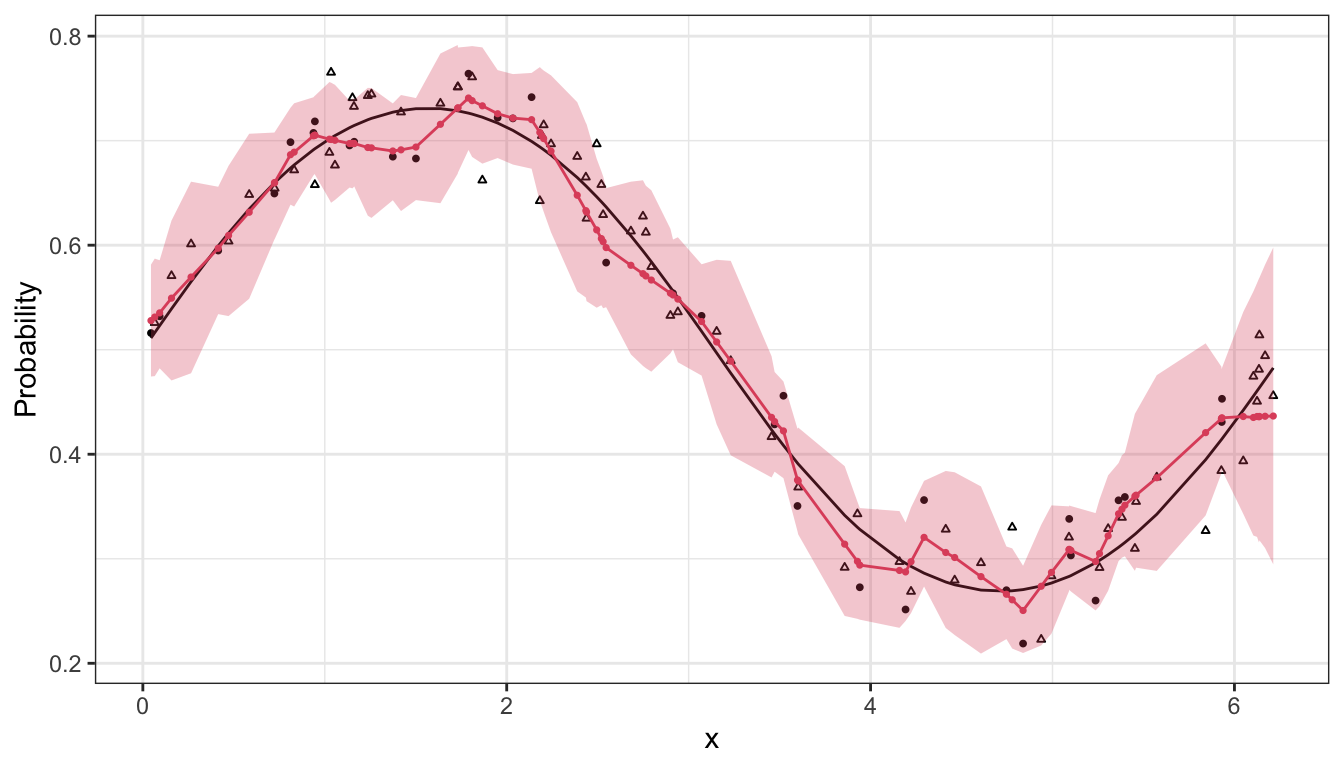
ggplot(d_obs, aes(x = x, y = plogis(eta))) +
  geom_line(lty = 1) +
  geom_point(data = d_obs[y_mis == 0],
             aes(x = x, y = y/n), size = 0.7) +
  geom_point(data = d_obs[y_mis == 1],
             aes(x = x, y = y/n), size = 0.7, pch = 2) +
  geom_ribbon(data = d_fig, 
              aes(x = x, ymin = q_025, ymax = q_975),
              inherit.aes = F, fill = 2, alpha = 0.3) +
  geom_line(data = d_fig, 
              aes(x = x, y = mu), col = 2) +
  geom_point(data = d_fig, 
              aes(x = x, y = mu), col = 2, size = 0.6) +
  scale_x_continuous("x") +
  scale_y_continuous("Probability") +
  theme_bw()

Figure 1: True function (black line), data on which the model was fit (black points), data we did not see (black triangles), random walk (red line) with interpolated points (red) and uncertainty (red ribbon).

Second order random walk

The second order random walk for regular locations has density

\[ \begin{aligned} \pi(x) \propto \exp\left( -\frac{1}{2} \sum_{i=2}^{n-1} (x_{i-1} - 2x_i + x_{i+1})^2 \right) \end{aligned} \]

The main term can be interpreted as an estimate of the second order derivative of a continuous time function. But this is not generally suitable for irregular spacings of x [1].

References

1. Lindgren F, Rue H. On the second-order random walk model for irregular locations. Scandinavian Journal of Statistics. 2008;35:691–700.